Poisson processes
The Poisson process is the mathematics of events that arrive “completely at random” in continuous time: order flow hitting a book, trades printing, jumps in a price path, buses (allegedly) arriving. From two innocuous axioms — independent, stationary increments — everything follows: Poisson counts, exponential gaps, the ability to split and merge streams, and a family of paradoxes that reward careful thinking.
Take a long interval and sprinkle points into it uniformly and independently — no clustering rule, no spacing rule, no memory. Now zoom into a subwindow: the count you see is binomial with tiny success probability, which is the Poisson limit derived in the distribution zoo. The Poisson process is this picture made rigorous, and its slogan is worth memorising: Poisson counts in time windows, exponential gaps between events, uniform positions given the count. Three descriptions, one process — practice problems are usually easy in exactly one of the three.
The counting-process definition#
A counting process counts events in : integer-valued, non-decreasing, . It is a Poisson process with rate if:
- Independent increments: counts over disjoint intervals are independent — what happened before says nothing about arrivals after .
- Stationary increments: the count over depends only on the length , not on where the window sits.
- Orderliness: in a sliver of length , and — events arrive one at a time.
These axioms force the marginal counts to be Poisson distributed:
Let . Split into and a sliver ; independence and orderliness give
Rearrange, divide by , and let : , with . The base case solves to , and induction (or the integrating factor ) climbs the ladder: . Alternatively: chop into slivers, each an independent Bernoulli() trial, and invoke the binomial-to-Poisson limit from the distribution zoo.
Worked example (by hand). Market orders hit a book at rate per minute. The probability of exactly 3 orders in the next 2 minutes uses :
And : quiet two-minute stretches happen about once an hour. Because mean equals variance, empirical counts that are overdispersed (variance greater than mean) are the standard evidence that real order flow clusters — the first crack the Poisson model shows in practice.
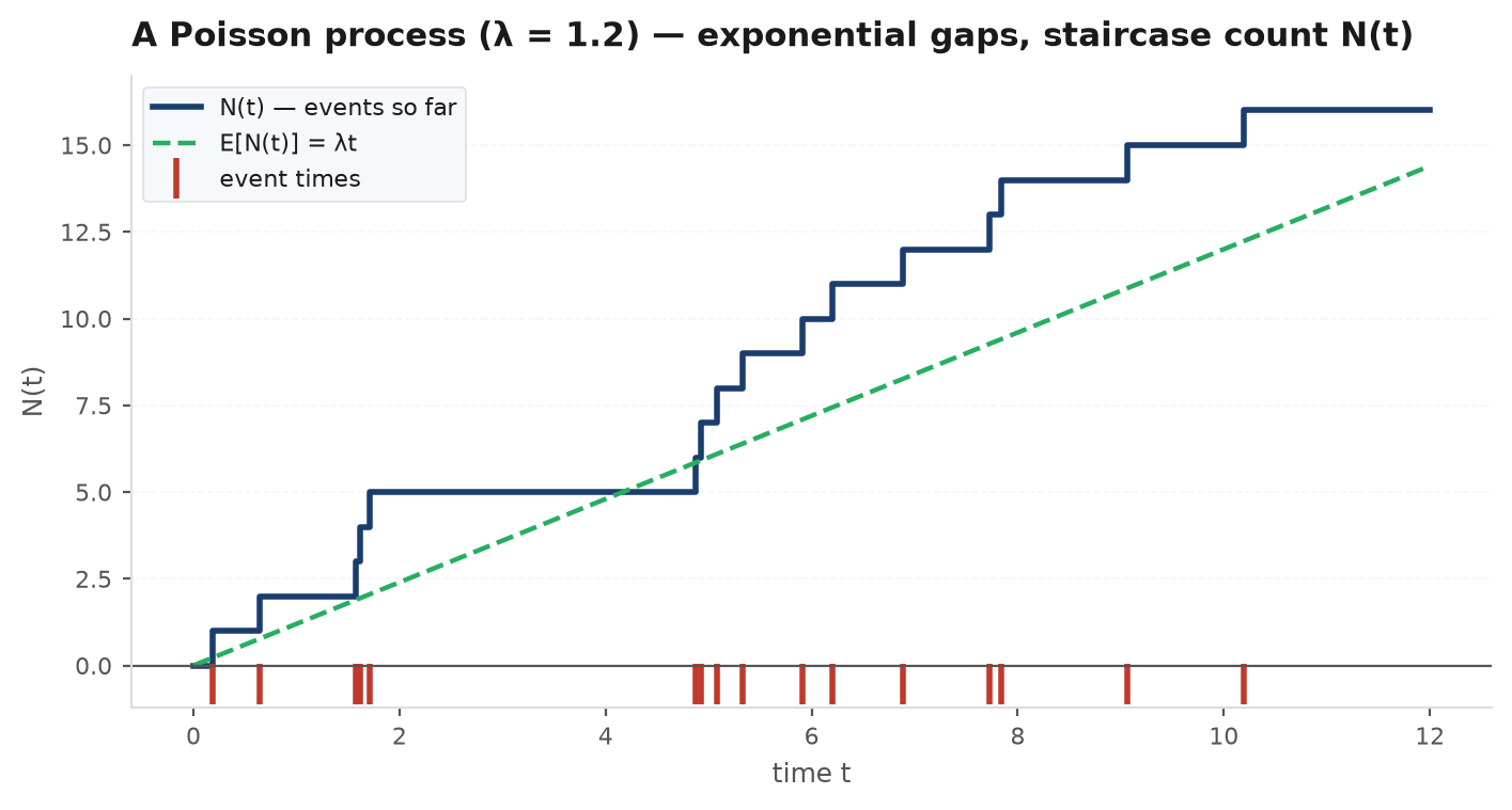
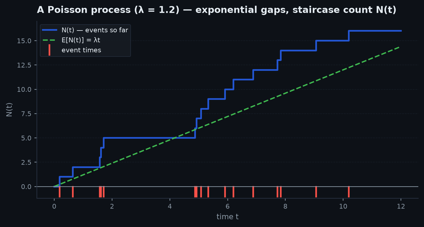
Interarrival times are exponential#
Let be the time of the first event. The event is exactly , so
By independent and stationary increments, the process restarts fresh at each arrival, so the gaps are iid . The converse also holds — laying down iid exponential gaps constructs a Poisson process — which is how you simulate one. The -th arrival time is a sum of iid exponentials, hence Erlang / Gamma:
That last identity — the -th arrival is early iff the count is high — converts arrival-time questions into count questions, and it is usually the fastest route by hand. Worked example: with /min, the probability the third order arrives within 2 minutes is
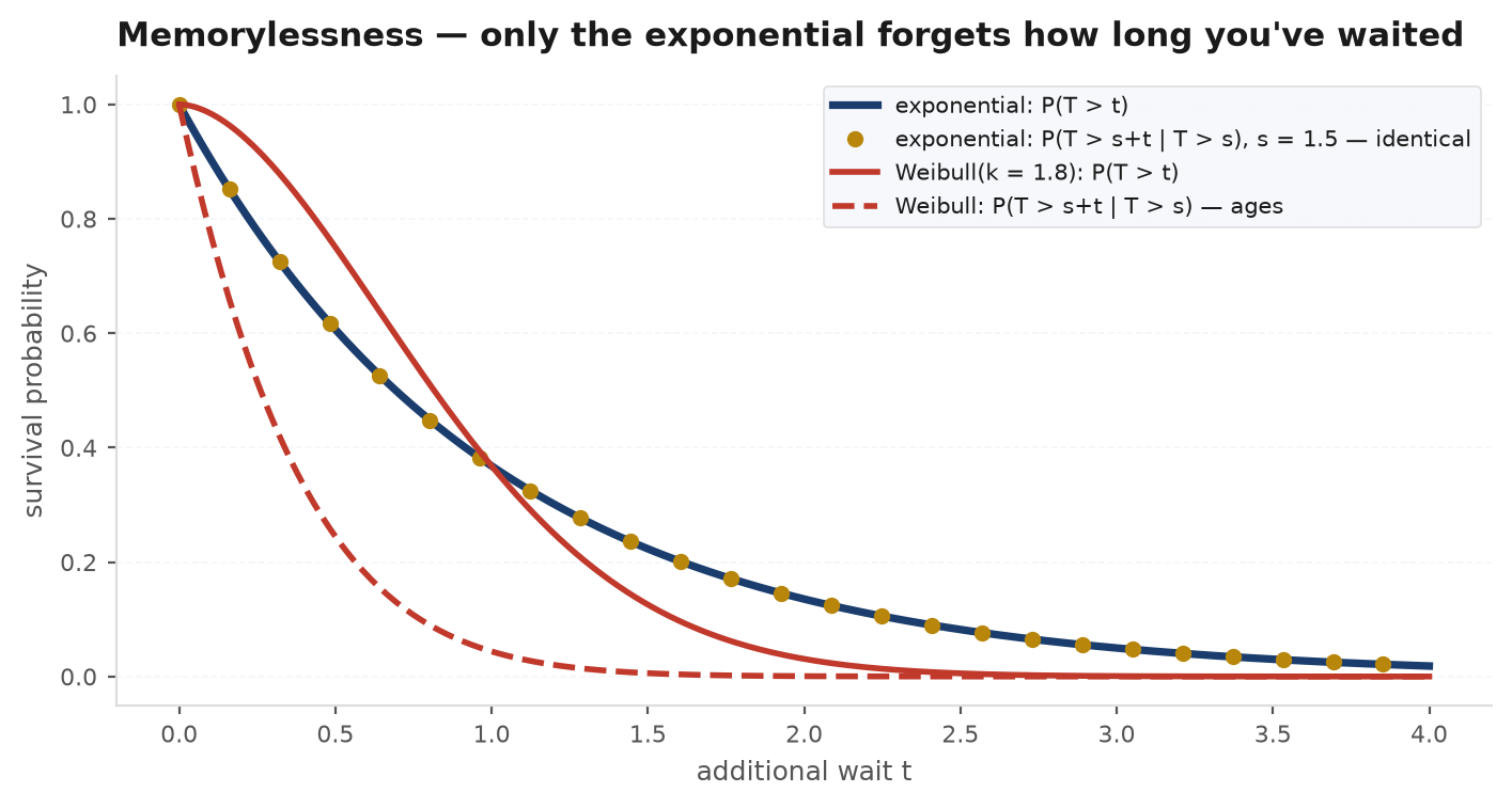
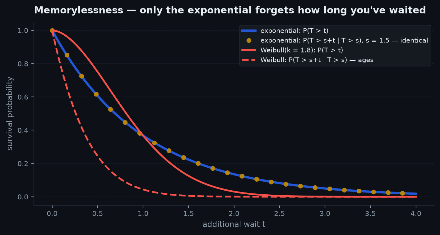
For and :
Having waited already changes nothing — the residual wait is a fresh . The exponential is the only continuous distribution with this property: memorylessness forces the survival function to satisfy , whose only right-continuous solutions are exponentials (Cauchy’s functional equation) — the uniqueness proof is spelled out in the distribution zoo. Memorylessness is the engine of nearly every problem below.
Superposition and thinning#
Poisson streams behave beautifully under merging and splitting. Superposition: if are independent Poisson processes with rates , then is Poisson with rate (independent stationary increments are inherited, and a sum of independent Poisson counts is Poisson — the MGF one-liner from the zoo). Thinning runs the other way: mark each arrival independently as type A with probability , type B otherwise.
Fix and let be the type counts in , with . Condition on the total and split the multinomial:
The joint pmf factorises into a Poisson() term times a Poisson() term — so the thinned counts are Poisson and independent, a genuinely surprising fact (knowing many buys arrived tells you nothing about how many sells did). The same computation over disjoint windows upgrades this to independence of the two processes.
Worked example (by hand). Orders arrive at 120 per hour; each is a buy with probability 0.55, independently. Buys form a Poisson process at /hour, sells at /hour, independent of each other. The probability of no sell in a given minute is — and learning that six buys printed in that minute would not change it.
Conditional uniformity#
The third face of the process: given , the arrival times are distributed as the order statistics of iid draws. Conditional on the count, the process carries no further structure — the points are just uniform dust. This converts many expectations into uniform-variable calculations. Worked example: 10 orders arrived in the last hour; the expected number in the first 15 minutes is , and the expected total “age” of the orders, , is order-minutes, since each arrival time is uniform with mean 30.
import numpy as np

rng = np.random.default_rng(11)
lam, T, reps = 2.0, 2.0, 100_000   # rate 2/min, 2-minute windows

# Build the process from iid exponential gaps; count arrivals in [0, T]
gaps = rng.exponential(1/lam, size=(reps, 40))
arrivals = np.cumsum(gaps, axis=1)
counts = (arrivals <= T).sum(axis=1)

print(counts.mean(), counts.var())          # both ~ lam*T = 4.0
print((counts == 3).mean())                 # ~ e^-4 * 4^3/3! = 0.1954

# Thinning: mark each arrival 'buy' w.p. 0.55 -> independent Poissons
marks = rng.random((reps, 40)) < 0.55
buys  = ((arrivals <= T) &  marks).sum(axis=1)
sells = ((arrivals <= T) & ~marks).sum(axis=1)
print(buys.mean(), sells.mean())            # ~ 2.2, 1.8
print(np.corrcoef(buys, sells)[0, 1])       # ~ 0.0  (independence!)
Compound Poisson: random sums#
Let jumps arrive as a Poisson process and give the -th jump a random size (iid, independent of the clock). The compound Poisson process is — total P&L from a random number of trades, total jump displacement of a price. Conditioning on the count (tower property and law of total variance, from joint distributions):
The variance collapses to — the second moment, not the variance, of the jump size — because Poisson mean equals variance. Worked example:100 trades/day, each with mean P&L $2 and standard deviation $50. Daily P&L has mean and variance , i.e. a daily sigma of about $500 — the trade-count randomness adds only the tiny term here, but for strategies with large mean-per-trade it dominates.
The inspection paradox#
Buses arrive as a Poisson process with rate , so gaps average . You show up at a “random” time. How long is the gap you land in? Not — on average it is twice that. Your arrival time is fixed, and a fixed point is more likely to land in a long gap: sampling intervals by throwing a dart at the timeline size-biases them.
If gaps have density and mean , an interval of length captures the dart with probability proportional to , so the gap you land in has the length-biased density , with mean . For : — exactly double. The memoryless decomposition says the same thing: the residual wait ahead of you is (mean ), and by time-reversal so is the age behind you; age plus residual gives mean . Only a perfectly regular schedule has zero size-bias; the factor grows with gap variability, which is why heavy-tailed service times make queues feel so much worse than their averages suggest.
The same size-biasing shows up whenever you sample by exposure: the class sizes students experience average more than the college’s mean class size, the drawdown you are currently in is longer than the typical drawdown, and the trade open when you glance at the book is likelier to be a slow one.
Practice problems#
Streams A and B are independent Poisson processes with rates and . What is the probability that exactly A-events occur before the first B-event?
Solution. Merge the streams: the superposition is Poisson with rate , and each event of the merged stream is independently an A with probability (thinning read backwards, or the min-of-exponentials fact of Problem 4). The question becomes: in a sequence of iid coin flips, probability of A’s then a B —
a geometric distribution. With : exactly two A’s first has probability . Continuous time has quietly disappeared — memorylessness reduces racing clocks to coin sequences, the single most reusable trick in this topic.
Buses arrive as a Poisson process, on average every 10 minutes. You arrive at a uniformly random time. What is your expected wait — and why is the naive answer of 5 minutes wrong?
Solution. Memorylessness answers instantly: whatever has happened, the time to the next bus is , so the expected wait is 10 minutes, not 5. The “half the average gap” intuition fails because you do not land in an average gap: you land in a length-biased one, mean minutes, and your expected position in it is halfway — . Both routes agree. For a deterministic 10-minute schedule the wait really is 5; the gap between 5 and 10 is purely the variance of the headways, with the coefficient of variation — a formula worth quoting.
For a Poisson process with rate , find .
Solution. Split the exponential series by parity. With :
Slicker: evaluate the probability generating function at . , and ; combined with the two summing to 1, the odd probability is . Note it is always below , approaching it as — the even side always keeps the head start from . The -at-a-special-point move recurs across many problems; file it next to the indicator trick from random variables.
Let and be independent. Find the distribution of and .
Solution. Survival functions multiply for independent minima:
For the race, integrate over the time of the minimum:
Rates behave like lottery tickets: the faster clock wins in proportion to its rate. Moreover the winner identity is independentof the winning time — the fact that lets Problem 1 treat the merged stream as iid coin flips. This trio (min is exponential at the summed rate; winner odds proportional to rates; independence of the two) is the complete toolkit for “which happens first” questions.
You enter a post office where two clerks are each serving a customer; you are next in line. Service times are iid . What is the probability you are the last of the three customers to leave?
Solution.You start service when the first of the two current services ends. At that moment, the other customer’s remaining service time is — by memorylessness — a fresh , exactly like yours. Two iid clocks, one race: . The tempting answer (“they had a head start, so more than 1/2”) is precisely the intuition memorylessness deletes. The same reasoning solves the light-bulb classic — a bulb that has burned 50 hours of an exponential mean-100-hour life has expected remaining life 100 hours, not 50 — and the follow-up : (wait for the first departure at the doubled rate, then your own service).
Next: from event clocks back to price paths — the simple random walk, the reflection principle, and its continuous limit, Brownian motion, with barrier-hitting results derived by martingale arguments. Random walks & Brownian motion.