Martingales & optional stopping

A martingale is a fair game made precise: given everything you know now, the expected next value is the current value. That single definition produces the most elegant machinery in probability — and some of the most useful in practice. The optional stopping theorem turns hard-looking questions (ruin probabilities, expected game lengths, waiting times for ABRACADABRA) into one-line equations; and its conditionsexplain, with full rigor, why no stop-loss, take-profit, or doubling scheme can conjure edge from a fair game. This chapter builds filtrations in plain language, proves optional stopping for bounded stopping times, solves gambler’s ruin both fair and biased, proves Wald’s identity, and walks the famous monkey-typing martingale.

✦Intuition — a fair game stays fair, no matter how cleverly you quit

Suppose each round of a game has zero expected profit. Can a clever exit rule— quit when ahead, double when behind, stop at the third loss — make the whole enterprise profitable? The optional stopping theorem says no, under conditions that amount to “you cannot wait forever and you cannot bet infinity.” Every apparent counterexample (the casino doubling system) works by violating exactly those conditions. For a trader the theorem is a null result of enormous value: if returns are a martingale, no overlay of stops and targets changes expectancy — so when a backtest improves after adding stops, the improvement came from non-martingale structure in the data (or from overfitting), never from the stop itself.

Filtrations, adaptedness, and the definition#

A filtration $F_{0} \subseteq F_{1} \subseteq \dots$ is simply the growing record of information: $F_{n}$ is everything observable by time $n$ (all coin flips so far, all prices so far). A process $M_{n}$ is adapted if $M_{n}$ is knowable at time $n$ — no peeking ahead. Then:

M_{n} is a martingale if E ∣ M_{n} ∣ < \infty and E [M_{n + 1} ∣ F_{n}] = M_{n} for all n .

Replace $=$ with $\geq$ for a submartingale (favourable game, drifting up) and $\leq$ for a supermartingale (unfavourable — mnemonic: supermartingales are what casinos offer you). Iterating the definition and using the tower property (joint distributions) gives $E [M_{n}] = E [M_{0}]$ for every fixed $n$ — the content of optional stopping is extending this to random times.

The three examples that solve ninety percent of problems — all built from i.i.d. steps $X_{i}$ with $S_{n} = X_{1} + \dots + X_{n}$ :

The walk itself: if $E [X_{i}] = 0$ , then $S_{n}$ is a martingale: $E [S_{n + 1} ∣ F_{n}] = S_{n} + E [X_{n + 1}] = S_{n}$ .
The compensated square: if additionally $Var (X_{i}) = σ^{2}$ , then $S_{n}^{2} - n σ^{2}$ is a martingale — expand $(S_{n} + X_{n + 1})^{2}$ : the cross term dies by independence, the $X_{n + 1}^{2}$ term contributes $σ^{2}$ , cancelled by the compensator. This one measures time.
The exponential (Wald) martingale: for any $θ$ where the MGF $M (θ) = E [e^{θ X}]$ exists, $Z_{n} = e^{θ S_{n}} / M (θ)^{n}$ is a martingale: $E [Z_{n + 1} ∣ F_{n}] = Z_{n} \cdot E [e^{θ X_{n + 1}}] / M (θ) = Z_{n}$ . Choosing $θ$ so that $M (θ) = 1$ kills the denominator — the trick that cracks biased random walks below. Products of independent mean-one terms (e.g. gross return relatives of a zero-drift asset) are the same construction.

Worked check (by hand). Fair coin steps $\pm 1$ : $M (θ) = cosh θ$ , so $e^{θ S_{n}} / cosh^{n} θ$ is a martingale for every $θ$ . For a biased walk with $P (X = + 1) = p$ , $P (X = - 1) = q$ , try $e^{θ} = q / p$ : then $M (θ) = p \cdot \frac{q}{p} + q \cdot \frac{p}{q} = q + p = 1$ , so

(\frac{q}{p})^{S_{n}} is a martingale — the key to biased gambler’s ruin.

→Quant lens — the martingale is the no-edge null

Weak-form market efficiency is the statement that (discounted) prices are a martingale with respect to the public filtration: $E [P_{t + 1} ∣ F_{t}] = P_{t}$ , i.e. expected return conditional on the past is zero. Every systematic strategy is a claim that this fails for some computable conditioning — and every backtest evaluation implicitly tests against this null (stochastic processes, why backtests lie). The optional stopping theorem sharpens the null: under it, no entry rule, exit rule, stop, or target — however path-dependent — has positive expectancy. Edges must come from the conditional mean, never from the choreography around it. That is why entries, exits & stops treats stops as risk-shaping tools, not alpha sources.

Stopping times and the optional stopping theorem#

A stopping time $τ$ is a random time whose arrival is decidable without foresight: ${τ \leq n} \in F_{n}$ for every $n$ . “First time the walk hits 10” is a stopping time; “the time the walk attains its eventual maximum” is not — you need the future to recognise it. (Most look-ahead bugs in backtests are, in this language, non-stopping-time exits.)

Optional stopping theorem: E [M_{τ}] = E [M_{0}] holds if any of: ⎩ ⎨ ⎧ (a) τ \leq K bounded; (b) τ < \infty a.s. and ∣ M_{n \land τ} ∣ \leq C; (c) E [τ] < \infty and ∣ M_{n + 1} - M_{n} ∣ \leq c .

✦Proof — optional stopping for bounded stopping times

Suppose $τ \leq K$ . Write the stopped value as a telescoping sum of increments taken only while the game is still running:

M_{τ} = M_{0} + n = 1 \sum K (M_{n} - M_{n - 1}) 1 {τ \geq n} .

The crucial observation: ${τ \geq n} = {τ \leq n - 1}^{c} \in F_{n - 1}$ — whether you are still playing at step $n$ was decided yesterday. So by the tower property,

E [(M_{n} - M_{n - 1}) 1 {τ \geq n}] = E [1 {τ \geq n} = 0 E [M_{n} - M_{n - 1} ∣ F_{n - 1}]] = 0,

and summing gives $E [M_{τ}] = E [M_{0}]$ . $■$ Cases (b) and (c) follow by applying this to $τ \land n$ (always bounded) and passing to the limit — dominated convergence for (b), and for (c) the bound $∣ M_{τ \land n} ∣ \leq ∣ M_{0} ∣ + c τ$ , integrable since $E [τ] < \infty$ . The proof is the trading statement: a stopped fair game is a sum of fair bets, each scaled by a decision made before the bet resolves.

!Counterexample — the doubling (martingale) betting system

Bet $1 on a fair coin; on each loss, double the stake; stop at the first win, $τ = min {n : X_{n} = win}$ . At $τ$ you have lost $1 + 2 + \dots + 2^{τ - 2} = 2^{τ - 1} - 1$ and won $2^{τ - 1}$ : wealth $W_{τ} = + 1$ , always. Yet $W_{n}$ is a martingale with $W_{0} = 0$ — so $E [W_{τ}] = 1 \neq = 0$ . Which hypothesis failed? $τ$ is finite a.s. and even $E [τ] = 2$ — but the increments are unbounded (stakes double) and the stopped process is unbounded below: before the redeeming win you are down $2^{n} - 1$ , which exceeds any credit line with positive probability. The “sure profit” is financed by an infinitely deep pocket that no one has; impose any finite bankroll and the rare wipeout exactly cancels the frequent small wins. Every martingale betting system, risk parity doubling grid, or “average down until saved” scheme dies on this same rock.

Gambler’s ruin — fair and biased, via optional stopping#

The canonical application. Start at $k$ (integer), take $\pm 1$ steps, stop at $τ$ = first hit of $0$ (ruin) or $N$ (target). The stopped walk is bounded in $[0, N]$ and $τ$ is a.s. finite with finite mean, so optional stopping applies in all uses below.

✦Derivation — fair case: hit probability and expected duration

Hit probability. $S_{n}$ is a martingale, so $E [S_{τ}] = k$ . But $S_{τ} \in {0, N}$ , so with $P = P (hit N first)$ :

N \cdot P + 0 \cdot (1 - P) = k ⟹ P = \frac{k}{N} .

Duration. Now stop the martingale $S_{n}^{2} - n$ : $E [S_{τ}^{2}] - E [τ] = k^{2}$ , and $E [S_{τ}^{2}] = N^{2} \cdot \frac{k}{N} = k N$ , so

E [τ] = k N - k^{2} = k (N - k) .

Start in the middle of $[0, 20]$ : even odds and $E [τ] = 100$ steps — the product form means games starting near an edge end fast, games starting centred last quadratically long.

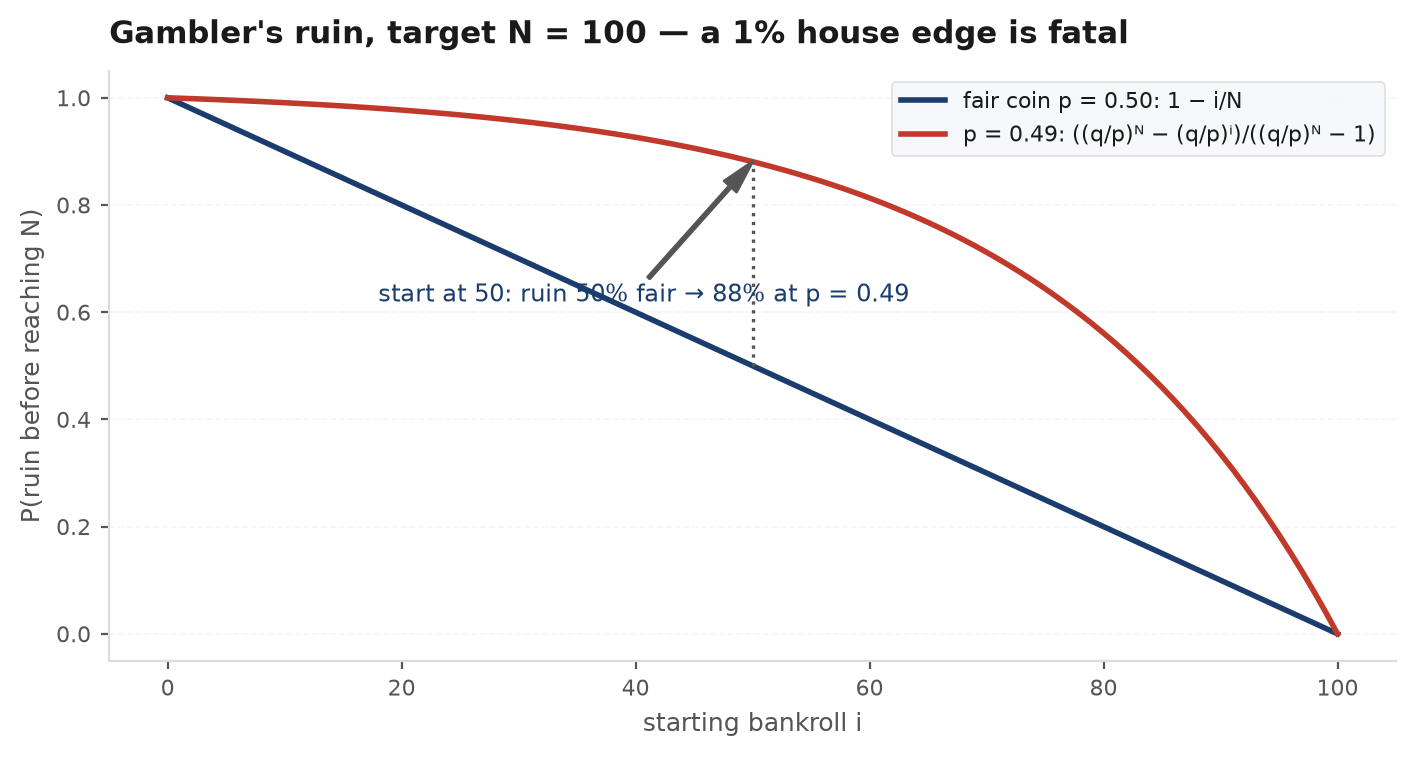
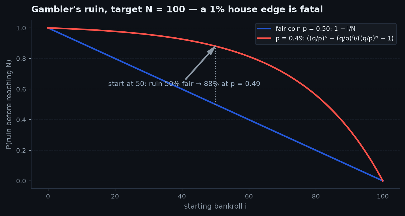
✦Derivation — biased case via the (q/p)^S martingale

Now $P (+ 1) = p \neq = \frac{1}{2}$ , $q = 1 - p$ , $r = q / p$ . Stop the martingale $r^{S_{n}}$ : $E [r^{S_{τ}}] = r^{k}$ gives $P r^{N} + (1 - P) r^{0} = r^{k}$ , so

P (hit N before 0) = \frac{1 - r ^{k}}{1 - r ^{N}}, r = \frac{q}{p} .

For the duration, stop the drift-compensated martingale $S_{n} - n (p - q)$ : $E [S_{τ}] - (p - q) E [τ] = k$ , hence

E [τ] = \frac{N P - k}{p - q}, P = \frac{1 - r ^{k}}{1 - r ^{N}} .

Worked numbers. $k = 10$ , $N = 20$ , $p = 0.49$ : $r = 51/49 \approx 1.0408$ , $r^{10} \approx 1.492$ , $r^{20} \approx 2.226$ , so $P = \frac{1 - 1.492}{1 - 2.226} \approx 0.401$ and $E [τ] = \frac{20 ( 0.401 ) - 10}{- 0.02} \approx 99$ . A 1% per-bet edge against you turns a 50/50 doubling shot into 40/60 — and the effect compounds catastrophically with distance: with $k = 100, N = 200$ the same tiny bias gives $P \approx 1.8%$ (Problem 4). Small edges, iterated, are destiny — the martingale-side proof of the casino arithmetic in LLN & the CLT.

Simulated gambler's ruin paths between absorbing barriers at zero and N, with the probability of reaching the target shown collapsing as the per-step bias turns negative — Gambler's ruin: random-walk paths between an absorbing floor (ruin) and ceiling (target). In the fair game the hit probability is the starting fraction k/N; with even a 1% per-step disadvantage the doubling probability collapses — (q/p)^S is the martingale that quantifies exactly how fast.

Wald’s identity#

Optional stopping applied to the drift-compensated walk deserves its own name, because it answers “how long, on average?” questions in one line.

✦Proof — Wald's identity

Let $X_{1}, X_{2}, \dots$ be i.i.d. with $E ∣ X ∣ < \infty$ , and $τ$ a stopping time with $E [τ] < \infty$ . Then

E [S_{τ}] = E [X] E [τ] .

Write $S_{τ} = \sum_{n = 1}^{\infty} X_{n} 1 {τ \geq n}$ . The event ${τ \geq n}$ is decided by $X_{1}, \dots, X_{n - 1}$ alone, hence independent of $X_{n}$ . Taking expectations term by term (Fubini, justified by $E [τ] < \infty$ ):

E [S_{τ}] = n \geq 1 \sum E [X_{n}] P (τ \geq n) = E [X] n \geq 1 \sum P (τ \geq n) = E [X] E [τ],

the last step being the tail-sum formula for expectations (random variables & moments). $■$

Worked example. Roll a fair die until the running total first reaches at least 300. Wald: $E [S_{τ}] = 3.5 E [τ]$ . The stopped total is 300 plus a small overshoot (renewal theory puts the average overshoot near $\frac{E [ X ^{2} ]}{2 E [ X ]} - \frac{1}{2} = \frac{91/6}{7} - \frac{1}{2} \approx 1.67$ ), so $E [τ] \approx 301.67/3.5 \approx 86.2$ rolls. The quant reading of Wald: expected P&L of a stopped strategy = (edge per trade) × (expected number of trades). Zero edge in, zero expectation out — whatever the stopping rule; and with positive edge, the way to earn more is to make $E [τ]$ — time in the game — larger, not to choreograph exits.

The ballot problem#

Theorem (Bertrand). In an election where A receives $a$ votes and B receives $b < a$ votes, counted in uniformly random order,

P (A strictly leads throughout the count) = \frac{a - b}{a + b} .

Sketch. The count is a lattice path of $+ 1$ s and $- 1$ s ending at $a - b > 0$ . Paths that touch zero after the first step can be reflectedabout the axis up to their first zero, giving a bijection between “bad” paths starting with an A-vote and all paths starting with a B-vote; a short count then leaves the fraction $(a - b) / (a + b)$ never tied. With $a = 60, b = 40$ : only $20%$ — even a landslide winner usually gets caught at least once. The reflection principle and its first-passage consequences are developed in random walks & Brownian motion; the martingale proof (via the backwards martingale $S_{k} / k$ ) is a beautiful second look.

ABRACADABRA — the monkey-typing martingale#

A monkey types i.i.d. uniform capital letters. What is the expected number of keystrokes until ABRACADABRA first appears? First-step recursions (Markov chains) work but drown in states. The martingale solution is one of the prettiest arguments in probability.

✦The betting-team argument, step by step

Just before each keystroke $n$ , a new gambler arrives with $1 and bets it on “the next letter is A.” Odds are fair (26-to-1 payout): winners hold $26 and let it ride on “next is B,” then “R,”… through the whole word; losers leave broke. Every individual bet is fair, so the team’s total wealth minus total stakes-paid-in is a martingale with bounded increments; the first-appearance time $τ$ has finite mean, so optional stopping (condition c) applies: $E [wealth at τ]$ = $E [stakes paid in] = E [τ]$ .

Now count the wealth at the moment ABRACADABRA completes. The gambler who started 11 letters ago rode the full word: $2 6^{11}$ . But she is not alone — any newer gambler whose partial ride matches a suffix of ABRACADABRA that is also a prefix survives too. The overlaps of ABRACADABRA with itself are ABRA (length 4) and A (length 1): the gambler 4 letters in holds $2 6^{4}$ , the one 1 letter in holds $26$ . Everyone else is broke. Hence

E [τ] = 2 6^{11} + 2 6^{4} + 26 \approx 3.67 \times 1 0^{15} .

The general rule: $E [τ] = \sum 2 6^{ℓ}$ over all $ℓ$ such that the length- $ℓ$ prefix equals the length- $ℓ$ suffix (including the full word). Self-overlap makes patterns slower to appear, because near-misses recycle progress for the pattern’s rivals, not for it — the same reason HH takes 6 fair-coin flips on average while HT takes only 4 (overlaps: $2^{2} + 2 = 6$ vs $2^{2} = 4$ ).

Azuma’s inequality is the concentration bound for martingales with bounded increments $∣ M_{n} - M_{n - 1} ∣ \leq c_{n}$ : $P (M_{n} - M_{0} \geq t) \leq exp (- t^{2} /2 \sum c_{k}^{2})$ — Hoeffding generalised to dependent-but-fair increments, and the rigorous form of “a zero-edge book with per-day risk limits cannot drift far” (tail bounds).

Sample paths of Brownian motion fanning out from zero with spread growing like the square root of time — Continuous-time martingale par excellence: Brownian motion. Both W_t and W_t^2 - t are martingales, so every discrete argument in this chapter — ruin probabilities via E[W_tau], durations via the compensated square — transfers verbatim to barrier-hitting problems for BM (see Problem 5).

ost_checks.py

import numpy as np

rng = np.random.default_rng(11)

def ruin(p, k, N, reps=20_000):
    """Simulate gambler's ruin: return (P(hit N first), E[steps])."""
    wins, steps = 0, 0
    for _ in range(reps):
        s, t = k, 0
        while 0 < s < N:
            s += 1 if rng.random() < p else -1
            t += 1
        wins += (s == N)
        steps += t
    return wins / reps, steps / reps

P, ET = ruin(0.50, k=10, N=20)
print(f"fair:   P(win)={P:.3f} (theory 0.500)   E[tau]={ET:.1f} (theory 100.0)")
P, ET = ruin(0.49, k=10, N=20)
print(f"biased: P(win)={P:.3f} (theory 0.401)   E[tau]={ET:.1f} (theory ~99)")

# Pattern waiting times: HH vs HT for a fair coin (overlap rule: 6 vs 4)
def wait(pattern, reps=100_000):
    total = 0
    for _ in range(reps):
        h, n = "", 0
        while not h.endswith(pattern):
            h += "HT"[rng.integers(2)]
            n += 1
        total += n
    return total / reps

print(f"E[wait HH] = {wait('HH'):.2f} (theory 6)   E[wait HT] = {wait('HT'):.2f} (theory 4)")

Practice problems#

→Problem 1 — the $10 gambler

You have $10, your opponent has $90. You bet $1 on fair coin flips until someone is broke. What is the probability you win everything?

Solution. Your wealth is a martingale stopped at $0$ or $100$ (bounded, so optional stopping applies cleanly): $100 \cdot P + 0 \cdot (1 - P) = 10$ , so $P = 10/100 = 0.1$ — your bankroll fraction, full stop. The slick framing to say out loud: a fair game preserves expected wealth, so probabilities of the two endings mustbe proportional to the distances, whatever the bet size pattern. Escalation to expect: “what if you can choose bet sizes?” Answer: still 0.1 — any adapted betting scheme keeps wealth a martingale (bold play changes the duration, not the probability, in a fair game).

→Problem 2 — how long does the game last?

Same setup: $10 vs $90, fair $1 bets. What is the expected number of bets until someone is broke?

Solution. Stop $S_{n}^{2} - n$ (unit-variance steps): $E [τ] = k (N - k) = 10 \times 90 = 900$ bets. The product structure is the discrete backbone of “variance measures time” — the same identity $E [W_{τ}^{2}] = E [τ]$ that gives stopped Brownian motion its clock (Problem 5), and why a fair book’s lifetime scales with the product of the distances to its risk limits, not their sum.

→Problem 3 — ABRACADABRA vs ABC

Monkey, uniform letters. Which appears sooner on average: ABC, or the same-length-11 word with no self-overlap, ABRACADABRZ — and how do both compare to ABRACADABRA?

Solution. By the betting-team argument, expected time = sum of $2 6^{ℓ}$ over self-overlap lengths $ℓ$ (full word included). ABC has no proper overlaps: $2 6^{3} = 17, 576$ . An 11-letter word with no self-overlap: $2 6^{11} \approx 3.67 \times 1 0^{15}$ . ABRACADABRA adds its ABRA and A overlaps: $2 6^{11} + 2 6^{4} + 26$ — longer than the overlap-free word of the same length, by a tiny relative amount with a crisp reason: when ABRACADABRA fails at the final A, the failing attempt cannot double as progress toward a fresh attempt, whereas its dangling ABRA-prefix survivors were counted as extra wealth the team must be paid for. The fair-coin miniature to quote: HH takes 6 flips, HT takes 4, even though both are 2-flip patterns with probability $1/4$ per placement.

→Problem 4 — doubling a bankroll at a 1% disadvantage

You start with 100 units and bet 1 unit per round at win probability $p = 0.49$ . What is the probability you reach 200 before 0?

Solution. Stop the martingale $(q / p)^{S_{n}}$ with $r = 0.51/0.49 \approx 1.0408$ :

P (200 before 0) = \frac{1 - r ^{100}}{1 - r ^{200}} \approx \frac{1 - 54.6}{1 - 2986} \approx 1.8%.

Against the fair-game answer of 50%: a 1% per-bet edge deficit destroys 96% of your doubling chances, because the exponent compounds the bias over the whole distance — $r^{100} = e^{100 l n r} \approx e^{4}$ . Points to volunteer: betting bigger helps when the odds are against you (10-unit bets make this the $k = 10, N = 20$ problem: $P \approx 40%$ ) — minimising the number of times the house edge taxes you; and symmetrically, when you have the edge, small bets and long games make winning nearly certain. That is bankroll management in one martingale, and the bridge to position sizing and the Kelly criterion.

→Problem 5 — Brownian motion hitting 1 before −2

$W_{t}$ is standard Brownian motion started at 0; $τ$ is the first time it hits $+ 1$ or $- 2$ . Find $P (W_{τ} = 1)$ and $E [τ]$ .

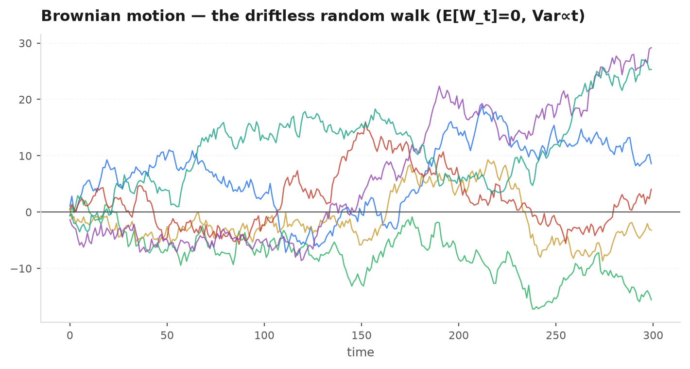
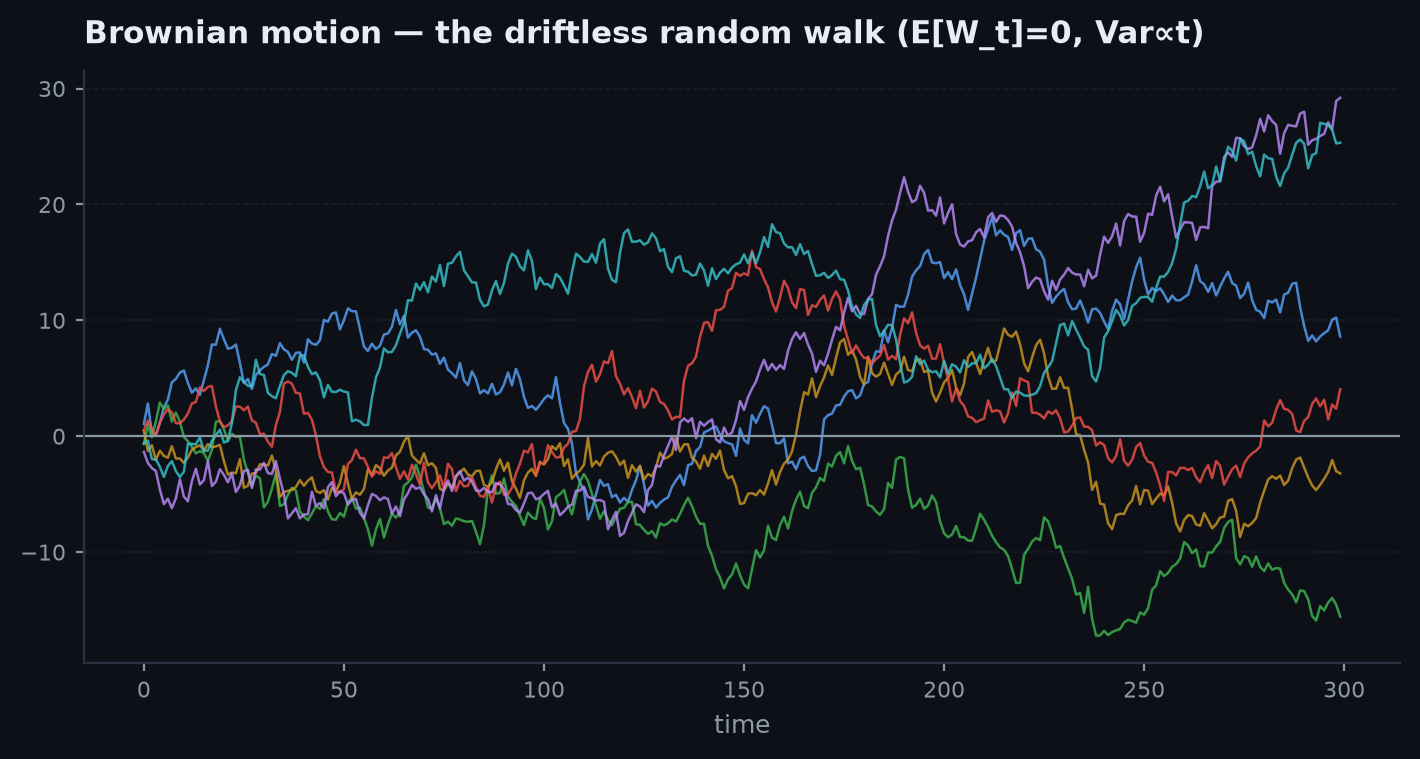
Solution. Both discrete arguments transfer verbatim. $W_{t}$ is a martingale and the stopped process is bounded in $[- 2, 1]$ : $0 = E [W_{τ}] = 1 \cdot P - 2 (1 - P)$ gives $P = 2/3$ — probabilities inversely proportional to barrier distances. $W_{t}^{2} - t$ is also a martingale: $E [W_{τ}^{2}] = E [τ]$ , and $E [W_{τ}^{2}] = \frac{2}{3} (1)^{2} + \frac{1}{3} (4) = 2$ , so $E [τ] = 2$ . In general: hit $a$ before $- b$ with probability $b / (a + b)$ , expected time $ab$ — the continuous gambler’s ruin, and the exact expected lifetime of a bracket order (stop at $- b$ , target at $a$ ) on a driftless diffusion. Note the expectancy check: $\frac{2}{3} (+ 1) + \frac{1}{3} (- 2) = 0$ — the bracket reshapes the distribution but cannot create edge, which is this whole chapter in one line.

Next: drop the fair-game requirement and keep only the memoryless structure — transition matrices, stationary distributions, and first-step analysis, the single most-used problem-solving technique: Markov chains.