Axioms, conditioning & Bayes

Three axioms generate all of probability theory. This chapter states them, derives their immediate consequences — complements, monotonicity, the union bound, continuity — and then builds the machinery of conditioning: the chain rule, the law of total probability, and Bayes’ theorem. Along the way it dissects Monty Hall properly, quantifies the base-rate fallacy with real numbers, and names the fallacies that cost traders money.

✦Intuition — why axioms, and why conditioning is the whole game

The axioms are bookkeeping: they guarantee probabilities behave like consistent proportions of belief, so you can compute without contradiction. The action is in conditioning. Every practical question — what is the chance of an edge given this backtest, of a fill given this book, of a crash given this vol regime — is a conditional probability. Problems in this area are rarely hard mathematically; they are hard because it is easy to condition on the wrong event, or to silently swap $P (A ∣ B)$ for $P (B ∣ A)$ . The cure is mechanical: write the sample space, write what you learned, cut down, renormalise.

Sample spaces, events, and σ-algebras#

A probability model has three parts. The sample space $Ω$ lists every possible outcome of the experiment — for two coin flips, $Ω = {H H, H T, T H, T T}$ . An event is a subset of $Ω$ — “at least one head” is ${H H, H T, T H}$ . The collection $F$ of events we assign probabilities to must be a σ-algebra: it contains $Ω$ , is closed under complement, and is closed under countable unions.

For finite spaces you can take all subsets and forget the issue. The concept earns its keep in continuous settings, where not every subset of $R$ can consistently be assigned a probability, and in stochastic processes, where a filtration — a growing family of σ-algebras $F_{t}$ — formalises “the information available by time $t$ ”. That idea carries the whole of martingales & optional stopping; here we only need the vocabulary.

The Kolmogorov axioms and their consequences#

A probability measure $P$ on $(Ω, F)$ satisfies exactly three axioms:

Non-negativity: $P (A) \geq 0$ for every event $A$ .
Normalisation: $P (Ω) = 1$ .
Countable additivity: for pairwise disjoint events $A_{1}, A_{2}, \dots$ , $P (\cup_{i} A_{i}) = \sum_{i} P (A_{i})$ .

Everything else is a theorem. The ones used daily:

P (A^{c}) = 1 - P (A), A \subseteq B \Rightarrow P (A) \leq P (B), P (A \cup B) = P (A) + P (B) - P (A \cap B) .

✦Proof — complement rule, monotonicity, and the union bound

Complement. $A$ and $A^{c}$ are disjoint with union $Ω$ , so additivity and normalisation give $P (A) + P (A^{c}) = 1$ . ■

Monotonicity. If $A \subseteq B$ , write $B = A \cup (B ∖ A)$ , disjoint. Then $P (B) = P (A) + P (B ∖ A) \geq P (A)$ by non-negativity. ■

Union bound (Boole’s inequality). Disjointify: let $B_{1} = A_{1}$ and $B_{i} = A_{i} ∖ (A_{1} \cup \dots \cup A_{i - 1})$ . The $B_{i}$ are pairwise disjoint, have the same union as the $A_{i}$ , and each $B_{i} \subseteq A_{i}$ . Then

P (i ⋃ A_{i}) = P (i ⋃ B_{i}) = i \sum P (B_{i}) \leq i \sum P (A_{i}) . ■

Crude but unconditional — it needs no independence, which is why it powers the Bonferroni correction in multiple testing: the chance that any of 20 null strategies clears $p < 0.0025$ is at most $20 \times 0.0025 = 5%$ , however correlated the strategies are.

✦Proof sketch — continuity of probability

If events increase, $A_{1} \subseteq A_{2} \subseteq \dots$ , then $P (\cup_{n} A_{n}) = lim_{n} P (A_{n})$ . Sketch: write the union as the disjoint union of rings $A_{1}, A_{2} ∖ A_{1}, A_{3} ∖ A_{2}, \dots$ ; countable additivity turns $P (\cup_{n} A_{n})$ into a telescoping series whose partial sums are exactly $P (A_{n})$ . The decreasing case follows by complements. ■This is the axiom-level fact behind statements like “a random walk hits every level eventually with probability 1” — you approximate the infinite-horizon event by finite-horizon ones and pass to the limit.

✦Worked example — axioms on a loaded die

A die is loaded so that $P (6) = 1/4$ and the other five faces are equally likely: each gets $(1 - 1/4) /5 = 3/20$ . Then $P (even) = P (2) + P (4) + P (6) = \frac{3}{20} + \frac{3}{20} + \frac{5}{20} = \frac{11}{20}$ by additivity, and $P (at most 5) = 1 - P (6) = 3/4$ by the complement rule. Mechanical — and that is the point: the axioms make every downstream computation an exercise in decomposition.

Conditional probability and the chain rule#

Learning that $B$ occurred shrinks the sample space to $B$ and renormalises:

P (A ∣ B) = \frac{P ( A \cap B )}{P ( B )}, P (B) > 0.

For fixed $B$ , the map $A \mapsto P (A ∣ B)$ is itself a probability measure — it satisfies all three axioms — so every theorem above applies verbatim after conditioning. Rearranging the definition and iterating gives the chain rule:

P (A_{1} A_{2} \dots A_{n}) = P (A_{1}) P (A_{2} ∣ A_{1}) P (A_{3} ∣ A_{1} A_{2}) \dots P (A_{n} ∣ A_{1} \dots A_{n - 1}) .

✦Worked example — two aces, by the chain rule

Draw two cards without replacement. $P (both aces) = P (A_{1}) P (A_{2} ∣ A_{1}) = \frac{4}{52} \cdot \frac{3}{51} = \frac{1}{221} \approx 0.45%$ . The chain rule is the formal version of “multiply along the tree,” and it is how the without-replacement dependence of the counting chapter gets priced in draw by draw.

The law of total probability#

Let $B_{1}, \dots, B_{n}$ partition $Ω$ — disjoint, with union $Ω$ , each with positive probability. Then for any event $A$ :

P (A) = i = 1 \sum n P (A ∣ B_{i}) P (B_{i}) .

✦Proof — decompose and apply additivity

The sets $A \cap B_{i}$ are pairwise disjoint (the $B_{i}$ are) and their union is $A \cap Ω = A$ . Countable additivity gives $P (A) = \sum_{i} P (A \cap B_{i})$ , and the definition of conditional probability rewrites each term as $P (A ∣ B_{i}) P (B_{i})$ . ■ In words: average the conditional probabilities, weighted by how likely each condition is. It is the probability-level version of the tower rule for expectations proved in joint distributions.

✦Worked example — a regime-mixture win rate

A breakout strategy wins 55% of trades in trending regimes and 35% in choppy ones; the market trends 40% of the time. Unconditional win rate: $P (W) = 0.55 \cdot 0.40 + 0.35 \cdot 0.60 = 0.22 + 0.21 = 0.43$ . Note what the law quietly enforces: the blended rate must lie between the conditional rates, weighted toward the more common regime. If your backtest shows 55% overall, you have implicitly assumed the market always trends — see regime detection for the applied version.

Bayes’ theorem#

Conditioning is asymmetric — $P (A ∣ B) \neq = P (B ∣ A)$ in general — and Bayes’ theorem is the exact exchange rate between the two directions:

P (B_{i} ∣ A) = \frac{P ( A ∣ B _{i} ) P ( B _{i} )}{P ( A )} = \frac{P ( A ∣ B _{i} ) P ( B _{i} )}{\sum _{j} P ( A ∣ B _{j} ) P ( B _{j} )} .

✦Proof — two definitions and one substitution

Write the definition of conditional probability in both directions for the same joint event: $P (B_{i} ∣ A) P (A) = P (A \cap B_{i}) = P (A ∣ B_{i}) P (B_{i})$ . Divide by $P (A)$ , then expand the denominator with the law of total probability over the partition ${B_{j}}$ . ■

The odds form is the version to compute with under pressure. For hypothesis $H$ and evidence $E$ :

posterior odds \frac{P ( H ∣ E )}{P ( H ^{c} ∣ E )} = prior odds \frac{P ( H )}{P ( H ^{c} )} \times likelihood ratio \frac{P ( E ∣ H )}{P ( E ∣ H ^{c} )} .

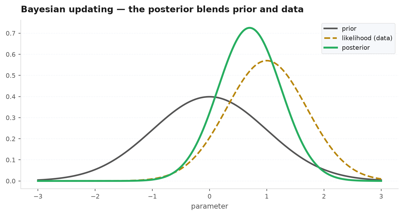
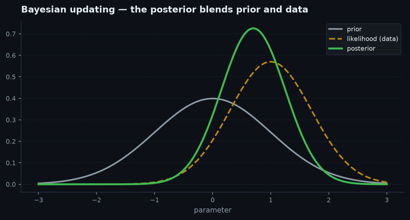
Multiply your prior odds by the likelihood ratio; done. Evidence with likelihood ratio 10 turns 1:99 odds into 10:99 — still an underdog. Sequential evidence just multiplies more ratios on, which is the engine of Bayesian inference and of the belief-updating chart below.

Posterior probability updating step by step as evidence accumulates, starting from a low prior — Bayesian updating in action: each piece of evidence multiplies the odds by its likelihood ratio, dragging the posterior from the prior toward certainty. Weak priors move fast; strong priors demand strong evidence — exactly how conviction in an edge should behave as live results accumulate.

The base-rate fallacy, with numbers#

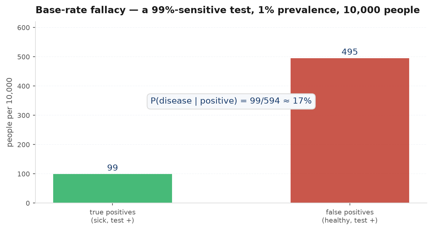
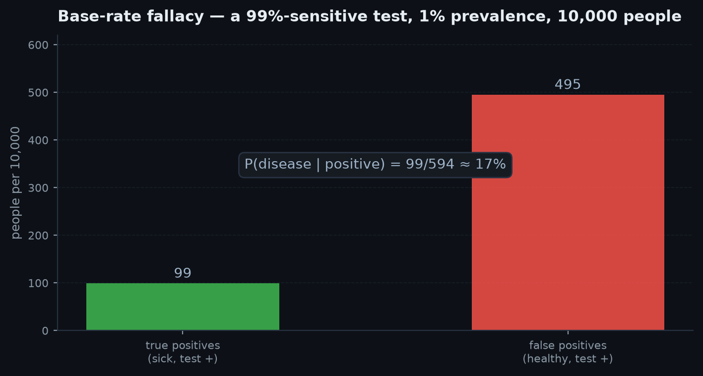
The classic: a disease affects 1% of the population. A test detects it 99% of the time when present (sensitivity) and gives a false positive 5% of the time when absent. You test positive. The tempting answer — “99% likely sick” — confuses $P (+ ∣ sick)$ with $P (sick ∣ +)$ . Bayes with a population of 10,000:

P (sick ∣ +) = \frac{0.99 \times 0.01}{0.99 \times 0.01 + 0.05 \times 0.99} = \frac{0.0099}{0.0099 + 0.0495} = \frac{99}{99 + 495} = \frac{1}{6} .

Of 10,000 people, 100 are sick and ~99 test positive; of the 9,900 healthy, ~495 also test positive. A positive result is five times more likely to come from the huge healthy pool than from the tiny sick one. The posterior is 16.7%, not 99% — the base rate dominates the test.

Population flow diagram showing that among all positive tests, false positives from the large healthy group outnumber true positives from the small sick group — The base-rate fallacy visualised on 10,000 people: the sick sliver (1%) yields 99 true positives, while the healthy mass yields 495 false positives. Among positives, only 99/594 ≈ 1 in 6 are actually sick. Rare condition + imperfect test = most alarms are false.

→Quant lens — your backtest is the medical test

Replace “sick” with “strategy has a real edge” and “positive test” with “great backtest.” True edges are rare (a low base rate), and flukes pass backtests at a non-trivial false-positive rate — so most impressive backtests are false positives, exactly as most positive tests above were healthy people. The arithmetic is worked as Problem 5 below, and the cure — demanding stronger evidence via permutation tests, walk-forward, out-of-sample —is the entire agenda of why backtests lie and the gauntlet. Bayes is not a topic in quant research; it is quant research.

Independence and conditional independence#

Events $A$ and $B$ are independent when $P (A \cap B) = P (A) P (B)$ — equivalently $P (A ∣ B) = P (A)$ : learning $B$ moves nothing. They are conditionally independent given $C$ when $P (A \cap B ∣ C) = P (A ∣ C) P (B ∣ C)$ . Neither notion implies the other, and both directions of failure matter:

Dependent, but conditionally independent. Pick a coin at random — one fair, one two-headed — and flip it twice. The flips are dependent (a first head raises the chance the coin is two-headed, hence the chance of a second head: $P (H_{2} ∣ H_{1}) = \frac{0.25 + 1}{0.5 + 1} = \frac{5}{6} > \frac{3}{4} = P (H_{2})$ ), yet given the cointhey are independent. Shared hidden causes create dependence — the reason “uncorrelated” strategies all drawing on the same regime crash together.
Independent, but conditionally dependent. Flip two fair coins; let $C$ be “at least one tail.” Unconditionally the flips are independent, but given $C$ , $P (H_{1} ∣ C) = 1/3$ while $P (H_{1} ∣ H_{2}, C) = 0$ . Conditioning on a common effectinduces dependence — Berkson’s paradox, formalised in multiple testing & paradoxes: select funds on (skill or luck) and, within the selected, skill and luck turn negatively related.

Monty Hall, in full#

Three doors: one car, two goats. You pick door 1. The host — who knows where the car is and always opens a goat door you did not pick — opens door 3. Switch to door 2 or stay?

Condition properly on the host’s action, not just “the car is not behind 3.” Let the car be at 1, 2, or 3 with prior $1/3$ each, and let $E$ = “host opens door 3”:

Car at 1 (you were right): host may open 2 or 3, so $P (E ∣ car 1) = 1/2$ .
Car at 2: host is forced to open 3, so $P (E ∣ car 2) = 1$ .
Car at 3: host never reveals the car, so $P (E ∣ car 3) = 0$ .

P (car 2 ∣ E) = \frac{1 \cdot \frac{1}{3}}{\frac{1}{2} \cdot \frac{1}{3} + 1 \cdot \frac{1}{3} + 0} = \frac{1/3}{1/2} = \frac{2}{3} .

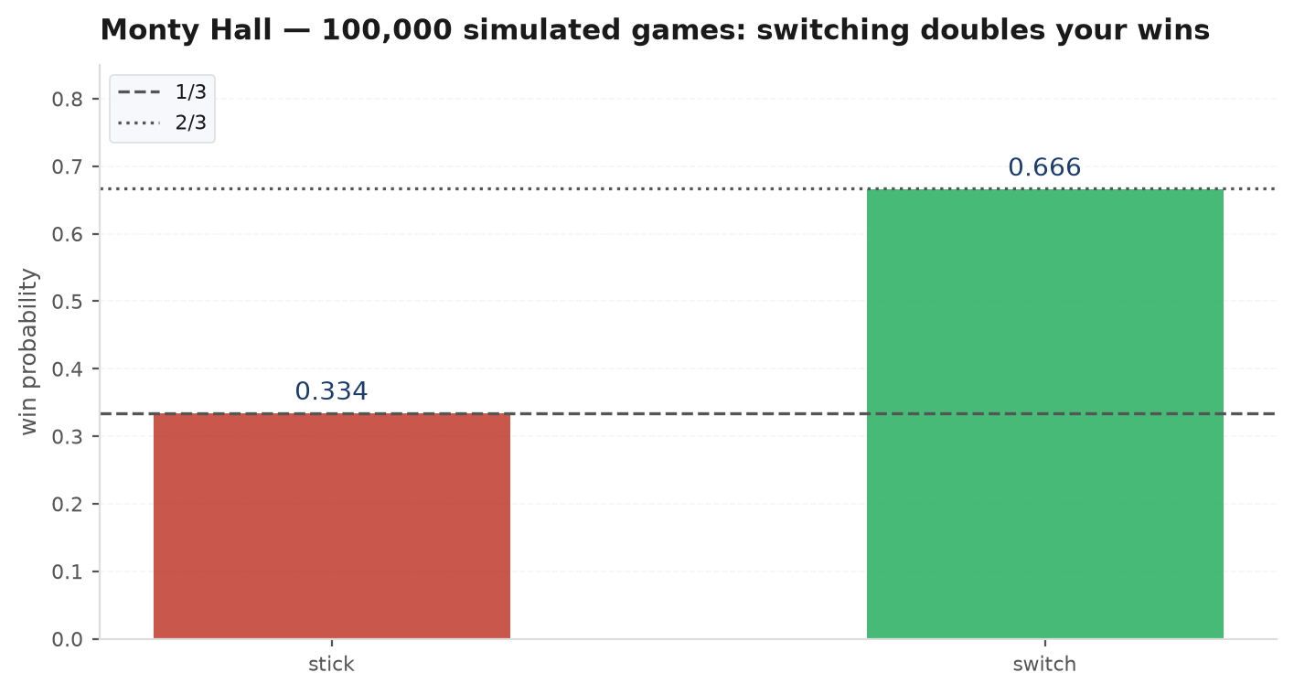
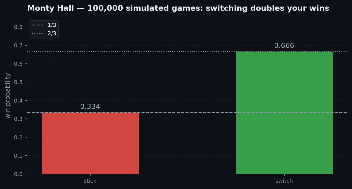
Switching wins with probability $2/3$ . The slick argument: your door wins iff your original pick was right — probability $1/3$ , untouched by the host’s show — so the remaining door carries the other $2/3$ . The information came from the host’s constraint: he was twice as likely to open door 3 when the car was at 2 (forced) as when it was at 1 (a coin toss), a likelihood ratio of 2 that turns prior odds 1:1 (door 1 vs door 2) into posterior odds 1:2.

Simulated win rates for the stay and switch strategies in Monty Hall converging to one third and two thirds — Monty Hall simulated: cumulative win rate of stay converges to 1/3 and switch to 2/3. The host's forced reveal is real information — conditioning on his action, not merely on 'door 3 has a goat', is what the naive 50/50 answer misses.

monty_hall_sim.py

import numpy as np

rng = np.random.default_rng(11)
trials = 100_000

car = rng.integers(0, 3, trials)          # where the car is
pick = rng.integers(0, 3, trials)         # your initial pick

# Host opens a goat door you didn't pick (forced when pick != car,
# random among the two goats when pick == car).
stay_wins = (pick == car)
# Switching wins exactly when your first pick was wrong:
switch_wins = ~stay_wins

print(f"stay   wins: {stay_wins.mean():.4f}   (theory 1/3 = 0.3333)")
print(f"switch wins: {switch_wins.mean():.4f}   (theory 2/3 = 0.6667)")
# Variant to try: a host who opens a random unpicked door (restart if it's
# the car) gives 50/50 — the forced-reveal mechanism is the whole answer.

!The assumptions are the answer

Change the host’s protocol and the answer changes. If the host opens a random unpicked door and it happens to show a goat, the likelihood ratio is 1 and switching is worth exactly $1/2$ — the “Monty Fall” variant. If the host only offers switches when you picked the car, switching always loses. Good prep questions probe precisely this: the answer $2/3$ is a consequence of the information-generating mechanism, not of the doors. Stating the protocol before computing is the mark of someone who actually understands conditioning.

Fallacies: gambler’s fallacy and Simpson preview#

The gambler’s fallacyexpects independent trials to self-correct: after five losses, a win is “due.” Independence says exactly the opposite — $P (W_{6} ∣ L_{1} \dots L_{5}) = P (W_{6})$ . What is true is that long-run frequencies converge (the LLN, in LLN & CLT) — by dilution of early outcomes, not compensation. Either trades are independent (a streak means nothing) or they are not (then model the dependence — Markov chains — rather than vibe it).

A second preview: aggregated and disaggregated conditional probabilities can point in opposite directions — a strategy can win within every regime yet lose overall if it concentrates exposure in the bad regime. That is Simpson’s paradox, dissected with numbers in multiple testing & paradoxes; the law of total probability above is the tool that resolves it.

Practice problems#

Five classics of conditioning — in each, the entire difficulty is identifying what you are conditioning on.

→Problem 1 — Two children, two ambiguities

A family has two children. (a) Given that at least one is a boy, what is the probability both are boys? (b) Given that at least one is a boy born on a Tuesday, what is the probability both are boys?

Solution. (a) Sample space of equally likely sex orders: ${B B, B G, GB, GG}$ . Conditioning removes $GG$ , leaving $B B$ among three: $1/3$ — not $1/2$ , because “at least one boy” is not “the first is a boy” (that conditioning gives $1/2$ ). (b) Count outcomes over sex × weekday (14 types per child). Families with a Tuesday boy: $1 4^{2} - 1 3^{2} = 27$ (complement count); of those, both-boys cases: $7^{2} - 6^{2} = 13$ . Answer: $13/27 \approx 0.481$ . The extra detail almost restores $1/2$ : the more specific the reported feature, the closer “at least one such child” comes to pointing at a particular child. The meta-lesson — how you learned a fact changes what it tells you— is Monty Hall’s lesson too.

→Problem 2 — Monty Hall with 100 doors

100 doors, one car. You pick one; the host, knowing the layout, opens 98 goat doors from the rest. Switch?

Solution. Your door retains its prior $1/100$ ; the host’s reveals are a deterministic show that squeezes the remaining $99/100$ onto the single unopened door. Switching wins with probability $99/100$ . This exaggerated version is the standard cure for 50/50 intuition — with the formal Bayes computation identical to the 3-door case: $P (E ∣ your door) = 1/99$ (host chose which door to leave shut at random) versus $P (E ∣ that door) = 1$ (forced), likelihood ratio 99.

→Problem 3 — A fair coin from a biased one (von Neumann)

You have a coin with unknown bias $p \in (0, 1)$ . Produce a fair 50/50 bit.

Solution. Flip twice. Output heads on $H T$ , tails on $T H$ , and discard-and-repeat on $H H$ or $T T$ . By independence, $P (H T) = p (1 - p) = P (T H)$ — the two accepted outcomes are exactly symmetric, so conditioned on acceptance each has probability $1/2$ regardless of $p$ . Expected flips: acceptance probability per round is $2 p (1 - p)$ , so $E [flips] = 2/ (2 p (1 - p)) = 1/ (p (1 - p))$ — 4 flips for a fair coin, worse as bias grows. The design pattern — manufacture symmetry, then condition on the symmetric subset — recurs across probability problems.

→Problem 4 — Die with no sixes: the all-even trap

Roll a fair die repeatedly until the first 6. Given that every roll in the sequence was even, what is the expected number of rolls?

Solution.The famous wrong answer is 3 — “given even rolls, it is a fair 3-sided die on ${2, 4, 6}$ , so geometric with $p = 1/3$ .” But conditioning on “allrolls even” is a statement about the whole sequence, and long sequences are less likely to stay even — the conditioning punishes length. Compute: $P (N = n, all even) = (2/6)^{n - 1} (1/6)$ (each pre-6 roll must be 2 or 4), so $P (all even) = \frac{1/6}{1 - 1/3} = \frac{1}{4}$ , and

E [N ∣ all even] = \frac{1}{P ( all even )} n \geq 1 \sum n (\frac{1}{3})^{n - 1} \frac{1}{6} = 4 \cdot \frac{1}{6} \cdot \frac{1}{( 1 - 1/3 ) ^{2}} = \frac{3}{2} .

Expected 1.5 rolls — shorter than the unconditional 6, and shorter even than the fake three-sided-die answer. Conditioning on a survival-type event reshapes the whole distribution; the same subtlety underlies survivorship bias in fund databases.

→Problem 5 — The false-positive trading signal

One strategy in fifty has a genuine edge. Your validation pipeline passes 90% of genuine edges and 10% of duds. A candidate passes. What is the probability it is genuine — and what after passing a second, independent validation?

Solution. Odds form. Prior odds: $1 : 49$ . Likelihood ratio of a pass: $0.90/0.10 = 9$ . Posterior odds $9 : 49$ , i.e. $P = 9/58 \approx 15.5%$ — a passing grade still means probably a dud. A second independent pass multiplies another 9: $81 : 49$ , giving $81/130 \approx 62%$ . Two lessons worth internalising: base rates make single confirmations weak, and independent evidence compounds multiplicatively in odds — why the gauntletstacks tests, and why “independent” matters: re-running a backtest on the same data multiplies by a likelihood ratio of 1.

Next: events and their probabilities become numbers and their distributions — expectation, variance, moment generating functions, and the indicator trick. Random variables & moments.