Gambler’s ruin & fair games

A gambler with a finite bankroll bets one unit at a time against a target: what is the chance of reaching it before going broke, and how long does the game last? This is the oldest problem in probability with a modern pulse — the exact mathematics of drawdown limits, prop-firm rules, and bet sizing. This chapter solves it three independent ways — first-step analysis, martingales, pure symmetry — because each method generalises in a different direction, then extracts the consequences: a fair game against a deep pocket is a losing game, ruin probability is exponentially sensitive to edge, and when the odds are against you the correct play is to bet big, not small.

✦Intuition — a linear resource against an exponential penalty

Hold two pictures. In a fair game, expected bankroll is conserved, so the probabilities of the two endings split in proportion to the distances: starting at $k$ out of $N$ , you reach the target with probability exactly $k / N$ — a straight line in $k$ . In a biased game, every unit of distance gets taxed by the same factor $q / p$ , and taxes on distance compound: the relevant quantity is $(q / p)^{k}$ , an exponentialin the bankroll. Linear resource, exponential penalty — that mismatch is why a 1–2% edge deficit, invisible in any single round, is catastrophic over a campaign, and why everything in this chapter reduces to controlling the exponent.

The setup and the two questions#

You start with a bankroll of $k$ units and play repeated one-unit bets: each round you win $+ 1$ with probability $p$ and lose $- 1$ with probability $q = 1 - p$ , rounds independent. The game stops when the bankroll first hits $0$ (ruin) or a target $N > k$ (success). In the language of Markov chains this is a birth–death chain on ${0, 1, \dots, N}$ with two absorbing states, and absorption is certain. Two questions carry everything:

Where does it end? $P_{k} = P (hit N before 0 ∣ start at k)$ .
How long does it take? $E [T_{k}]$ , the expected number of rounds until absorption.

The problem made a cameo in martingales & optional stopping; here it gets the dedicated treatment, solved three ways on purpose — the same answer from a difference equation, a stopped martingale, and a conservation law is how you know the answer.

Method 1 — first-step analysis#

Condition on the first bet, exactly as in the first-step analysis of Markov chains. From state $k$ you move to $k + 1$ with probability $p$ or $k - 1$ with probability $q$ , and the memoryless structure restarts the problem from the new state:

P_{k} = p P_{k + 1} + q P_{k - 1}, 1 \leq k \leq N - 1, P_{0} = 0, P_{N} = 1.

✦Proof — solving the difference equation by telescoping

Since $p + q = 1$ , rewrite the left side as $(p + q) P_{k}$ and regroup:

p (P_{k + 1} - P_{k}) = q (P_{k} - P_{k - 1}) ⟹ d_{k} = (\frac{q}{p}) d_{k - 1}, d_{k} := P_{k + 1} - P_{k} .

The successive differences form a geometric sequence, $d_{k} = r^{k} d_{0}$ with $r = q / p$ (equivalently: the characteristic equation $p x^{2} - x + q = 0$ has roots $1$ and $q / p$ , so the general solution is $A + B r^{k}$ ). Telescope from $P_{0} = 0$ :

P_{k} = j = 0 \sum k - 1 d_{j} = d_{0} (1 + r + \dots + r^{k - 1}) = d_{0} \frac{r ^{k} - 1}{r - 1} (r \neq = 1) .

The other boundary $P_{N} = 1$ fixes $d_{0} = (r - 1) / (r^{N} - 1)$ , giving the biased-game answer; when $r = 1$ (fair game) the differences are all equal, so $P_{k} = k d_{0}$ and $P_{N} = 1$ forces $d_{0} = 1/ N$ . ■

P_{k} = ⎩ ⎨ ⎧ \frac{k}{N}, \frac{1 - ( q / p ) ^{k}}{1 - ( q / p ) ^{N}}, p = \frac{1}{2}, p \neq = \frac{1}{2} .

Sanity checks: as $p \to \frac{1}{2}$ the biased formula collapses to $k / N$ (all differences become equal) — the fair case is the limit, not a separate universe — and your opponent’s success probability (start $N - k$ , win-probability $q$ ) plus yours sums to 1: absorption is certain, nobody plays forever.

Method 2 — martingales: two-line answers#

With the optional stopping theorem in hand from martingales & optional stopping, both cases collapse to one substitution each. Let $S_{n}$ be the bankroll and $τ$ the absorption time; the stopped process is bounded in $[0, N]$ with $E [τ] < \infty$ , so stopping is legal throughout.

Fair case. $S_{n}$ is itself a martingale, so $E [S_{τ}] = k$ . But $S_{τ} \in {0, N}$ , so $N P_{k} = k$ , i.e. $P_{k} = k / N$ .
Biased case. $(q / p)^{S_{n}}$ is the exponential martingale (the MGF-killing choice $e^{θ} = q / p$ ), so $E [r^{S_{τ}}] = r^{k}$ with $r = q / p$ : $P_{k} r^{N} + (1 - P_{k}) = r^{k}$ , which rearranges to $P_{k} = (1 - r^{k}) / (1 - r^{N})$ .

Same answers, a tenth of the work. First-step analysis needs no theory and survives state-dependent transition probabilities; the martingale route needs machinery but transfers verbatim to continuous time, pricing barrier-hitting for Brownian motion in the same two lines (random walks & Brownian motion).

Method 3 — symmetry: no free lunch in a fair game#

The fair case needs no computation at all. A fair bet conserves expected wealth; a sequence of fair bets, stopped by any rule that cannot see the future, still conserves it. Your expected final bankroll therefore equals your starting bankroll. But the final bankroll is either $0$ or $N$ — nothing in between survives — so

P_{k} \cdot N + (1 - P_{k}) \cdot 0 = k ⟹ P_{k} = \frac{k}{N} .

Read it as a no-free-lunch statement: in a fair game, the probability of multiplying your stake by $N / k$ is exactly $k / N$ — probability times payoff multiple equals one, always. No bet-sizing pattern, stopping rule, or streak-reading system moves it, because any adapted scheme keeps wealth a martingale. Every claimed system for beating a fair game hides an assumption of infinite credit somewhere — dissected as the doubling-system counterexample in the martingale chapter.

How long does the game last?#

First-step analysis answers the duration question with the same move: condition on round one, which costs one round and restarts the clock from the new state.

E [T_{k}] = 1 + p E [T_{k + 1}] + q E [T_{k - 1}], E [T_{0}] = E [T_{N}] = 0.

✦Proof — the fair-case duration is k(N − k)

With $p = q = \frac{1}{2}$ the recursion says the second difference of $E [T_{k}]$ is constant: $E [T_{k + 1}] - 2 E [T_{k}] + E [T_{k - 1}] = - 2$ . A particular solution is $- k^{2}$ ; the homogeneous solutions are $a + bk$ ; so $E [T_{k}] = - k^{2} + a + bk$ . The boundaries $E [T_{0}] = 0$ and $E [T_{N}] = 0$ force $a = 0$ , $b = N$ :

E [T_{k}] = k (N - k) . ■

The martingale route lands the same place in one line — stop $S_{n}^{2} - n$ ; Wald’s second identity is the same fact under another name. For the biased game, stop the drift-compensated walk $S_{n} - n (p - q)$ instead: $E [T_{k}] = (N P_{k} - k) / (p - q)$ .

The size of the fair-case answer is the striking part. Trying to double 50 into 100 by unit bets: $E [T] = 50 \times 50 = 2, 500$ rounds. The product form $k (N - k)$ says games starting near a barrier end fast while centred games last quadratically long — diffusion covers distance like $t$ , so distance $d$ costs time of order $d^{2}$ . A fair game is not just unprofitable in expectation; it is a spectacular waste of time.

The infinitely rich opponent#

Now let the opponent be a casino, a market, or anyone whose bankroll you cannot exhaust: send $N \to \infty$ and ask for the probability of escaping ruin forever.

Fair game ( $p = \frac{1}{2}$ ): $P_{k} = k / N \to 0$ . Ruin is certain.
Unfavourable game ( $p < \frac{1}{2}$ ): $r = q / p > 1$ , so $P_{k} = (1 - r^{k}) / (1 - r^{N}) \to 0$ . Ruin is certain, and faster.
Favourable game ( $p > \frac{1}{2}$ ): $r < 1$ , so $r^{N} \to 0$ and $P (never ruined) = 1 - r^{k} = 1 - (q / p)^{k}$ . Ruin probability $(q / p)^{k}$ , exponentially small in the bankroll.

The first bullet deserves a pause, because it violates most people’s intuition about the word “fair.” Round by round you are not being cheated; yet against a deep enough pocket you lose everything with probability 1. The mechanism: the fair walk is recurrent — it will visit 0 eventually — and once your target is removed, the only absorbing state left is your ruin. A fair game against an infinitely rich adversary is a losing game; the casino does not even need its house edge to beat a patron who keeps playing — the edge just collects the inevitable sooner. On the favourable side: $p = 0.55$ with $k = 10$ gives ruin probability $(9/11)^{10} \approx 0.134$ — a genuine 10-point edge still loses everything 13.4% of the time when the bankroll is only ten bets deep.

Sensitivity to edge: why 1% is catastrophic#

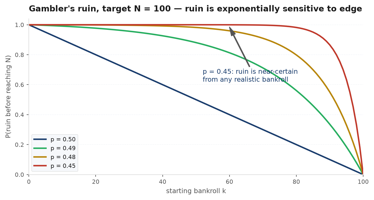
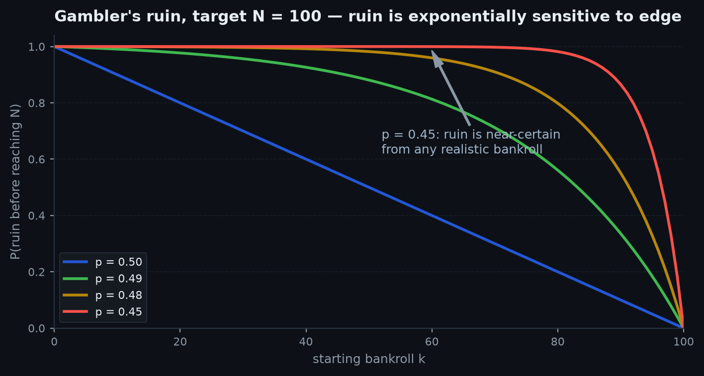
Fix $k = 50$ , $N = 100$ — a campaign to double a bankroll — and dial the win probability down by steps a single session could never detect:

P (ruin) : p = 0.50 \Rightarrow 50%, p = 0.49 \Rightarrow 88.1%, p = 0.48 \Rightarrow 98.2%, p = 0.45 \Rightarrow 99.996%.

A one-point deficit nearly doubles the ruin probability; two points make success a 1-in-56 shot; five points, 1-in-23,000. The mechanism is the exponent: for $p$ near $\frac{1}{2}$ , $ln (q / p) \approx 2 (q - p)$ , so

(\frac{q}{p})^{k} \approx e^{2 (q - p) k} — the edge deficit is multiplied by the whole distance before being exponentiated.

At $p = 0.49$ the per-round tax is 2 cents on the dollar, but over $k = 50$ units of distance the exponent is $2 \times 0.02 \times 50 = 2$ , and $e^{2} \approx 7.4$ already dominates the arithmetic. Edges do not add across a campaign; they compound.

Ruin probability as a function of starting bankroll k for win probabilities 0.50, 0.49, 0.48 and 0.45 with target 100, showing the fair-game straight line against biased curves collapsing toward certain ruin — Ruin probability against starting bankroll k for a target of N = 100. The fair game is the straight line 1 − k/N; every biased curve bows toward certain ruin, and by p = 0.45 the curve hugs 100% until k is nearly the whole target. The gap between curves is governed by (q/p)^k ≈ e^{2(q−p)k} — ruin probability responds exponentially, not linearly, to the per-round edge.

ruin_check.py

import numpy as np

rng = np.random.default_rng(21)

def theory(p, k, N):
    """Closed-form (ruin probability, expected duration)."""
    if p == 0.5:
        return 1 - k / N, k * (N - k)
    r = (1 - p) / p
    win = (1 - r**k) / (1 - r**N)
    return 1 - win, (N * win - k) / (2 * p - 1)

def simulate(p, k, N, reps=20_000):
    """Vectorised gambler's ruin: (ruin frequency, mean duration)."""
    s = np.full(reps, k)
    active = (s > 0) & (s < N)
    steps = 0
    while active.any():
        n = active.sum()
        s[active] += np.where(rng.random(n) < p, 1, -1)
        steps += n
        active = (s > 0) & (s < N)
    return (s == 0).mean(), steps / reps

k, N = 50, 100
print(f"{'p':>5} | {'ruin sim':>9} {'ruin theory':>12} | {'E[T] sim':>9} {'E[T] theory':>12}")
for p in (0.50, 0.49, 0.48, 0.45):
    r_sim, t_sim = simulate(p, k, N)
    r_th, t_th = theory(p, k, N)
    print(f"{p:>5.2f} | {r_sim:>9.4f} {r_th:>12.4f} | {t_sim:>9.1f} {t_th:>12.1f}")
# Expected: ruin 0.5000 / 0.8808 / 0.9821 / ~1.0000; fair-case duration 2,500.

Bold play vs timid play#

Bet size is a free parameter the formulas price exactly: betting $b$ units per round is the unit-bet problem with $k / b$ and $N / b$ — rescaling shrinks the exponent. The consequence is a rule most people find backwards: when the game is unfavourable, bet big; when it is favourable, bet small. Each round of a negative-edge game is another chance for the house to collect its tax; subdividing a campaign into many small bets maximises the number of collections, and bold play minimises them.

✦Worked example — turning 50 into 100 at p = 0.47

Target: double a 50-unit bankroll at win probability $p = 0.47$ ( $r = 53/47 \approx 1.1277$ ).

Timid — unit bets ( $k = 50, N = 100$ ): $P = \frac{1 - r ^{50}}{1 - r ^{100}} = \frac{1 - 406}{1 - 165 , 000} \approx 0.0025$ — a 0.25% chance.
Medium — 10-unit bets ( $k = 5, N = 10$ ): $P = \frac{1 - r ^{5}}{1 - r ^{10}} = \frac{1 - 1.823}{1 - 3.325} \approx 0.354$ — 35.4%.
Bold — one double-or-nothing bet ( $k = 1, N = 2$ ): $P = \frac{1 - r}{1 - r ^{2}} = \frac{1}{1 + r} = p = 0.47$ — 47%.

Same game, same goal, and the win probability spans a factor of nearly 190 purely through stake size: the single maximal bet exposes the edge deficit exactly once, while grinding is maximally ruinous. Flip the edge and everything reverses — at $p = 0.53$ , unit bets succeed $\approx 99.75%$ of the time while the bold bet wins only 53%: with an edge you want the LLN grinding for you, in many small installments (LLN & CLT). In the exactly fair game size does not matter: $P = k / N$ at every stake — bet size buys duration, never probability.

Quant lens — risk of ruin for traders#

Translate the board game into a trading account. Measure everything in R-multiples — one R is the amount risked per trade — with each trade winning $+ 1 R$ with probability $p$ or losing $- 1 R$ with probability $q$ . A drawdown limit — yours, or one imposed by a prop firm — sits $D$ percent below starting equity. The distance to ruin is then $k = D / f$ units, where $f$ is the fraction risked per trade, and the probability of ever breaching the limit while trading toward an open-ended upside is exactly the infinite-opponent formula:

P (breach) = (\frac{q}{p})^{k} = (\frac{q}{p})^{D / f} (p > \frac{1}{2}) .

Every term is a lever. Risking $f = 2%$ against a $D = 10%$ limit gives $k = 5$ — a prop trader is a gambler five bets from the rail, whatever the account’s notional size. Halving the risk per trade doubles $k$ and therefore squares the ruin probability: a 36.7% breach risk becomes 13.4% (Problem 5). That squaring law is the practical content of this chapter for position sizing: size is not a linear dial on risk of ruin, it is an exponent. The growth-optimal resolution of the trade-off is the Kelly criterion, developed there too — full Kelly maximises expected log growth, and any fixed fraction of it buys exponentially better ruin protection at a linear cost in growth rate. And note which side of the table an edge puts you on: you are the house — small bets, long games, let the exponent work for you.

!The formulas assume i.i.d. bets of fixed size

Everything above is exact for independent, identically distributed bets with a constant stake — and real trading violates all three clauses. Serial correlation makes losing streaks longer than the i.i.d. arithmetic allows, effectively shrinking $k$ ; volatility clustering means “1R” is not constant precisely when it matters; fat-tailed fills can lose several R in one step, jumping over the barrier arithmetic entirely. Treat $(q / p)^{k}$ as an optimistic floor on ruin risk, not an estimate — and test the dependence structure before trusting it, with the tools of time-series statistics.

Practice problems#

Five problems to test understanding — one workout per method or consequence, numbers carried to the end.

→Problem 1 — unequal stakes, fair game

You have 10 units, your opponent has 15; you bet one unit per round on a fair coin until someone is broke. Find your probability of winning everything and the expected length of the game.

Solution. Here $k = 10$ , $N = 10 + 15 = 25$ . By the conservation argument (Method 3), your win probability is your share of the total capital: $P = k / N = 10/25 = 0.4$ ; ruin probability $0.6$ ; duration $E [T] = k (N - k) = 10 \times 15 = 150$ rounds. Takeaway: in a fair game the capital split isthe probability split — the richer player wins more often only because the poorer player’s barrier is closer — and the duration is the product of the two distances, not their sum.

→Problem 2 — the same game with a 1% edge deficit

Same stakes — $k = 10$ , $N = 25$ — but now $p = 0.49$ . Compute your success probability and compare it to the fair answer.

Solution. $r = q / p = 51/49 \approx 1.0408$ , so $r^{10} \approx 1.492$ , $r^{25} \approx 2.719$ , and

P = \frac{1 - r ^{10}}{1 - r ^{25}} = \frac{1 - 1.492}{1 - 2.719} = \frac{0.492}{1.719} \approx 0.286.

The fair game gave 40%; a one-point edge deficit strips more than a quarter of the winning chances (28.6%), while the expected duration barely moves: $E [T] = (25 \times 0.286 - 10) / (0.49 - 0.51) \approx 142$ rounds against the fair 150. Takeaway: small bias barely changes how long you play but dramatically changes where you end up — drift acts on the destination, variance on the clock.

→Problem 3 — deriving the fair-game clock

Derive $E [T_{k}] = k (N - k)$ for the fair game directly from the difference equation, and verify it at $k = 50$ , $N = 100$ .

Solution. The recursion $E [T_{k}] = 1 + \frac{1}{2} E [T_{k + 1}] + \frac{1}{2} E [T_{k - 1}]$ rearranges to a constant second difference $Δ^{2} E [T_{k}] = - 2$ — the discrete analogue of $u^{''} = - 2$ . Integrate twice: $- k^{2}$ plus the linear homogeneous family $a + bk$ ; the boundaries $E [T_{0}] = E [T_{N}] = 0$ give $a = 0, b = N$ , hence $E [T_{k}] = k (N - k)$ ; at $k = 50$ , $50 \times 50 = 2, 500$ rounds. Cross-check by stopping $S_{n}^{2} - n$ : $E [T] = k N - k^{2}$ — same answer, two roads. Takeaway: absorbing-barrier durations solve a discrete Poisson equation; recognising the shape turns these from memorised formulas into thirty-second derivations.

→Problem 4 — escaping an infinitely rich opponent

You play an infinitely rich adversary with a real edge: $p = 0.52$ , starting bankroll $k = 20$ . What is the probability you are never ruined? What does the answer become at $p = 0.50$ , and at $k = 40$ ?

Solution. Escape probability $1 - (q / p)^{k}$ with $q / p = 48/52 = 12/13$ : $(12/13)^{20} = e^{20 l n (12/13)} \approx e^{- 1.601} \approx 0.202$ , so you survive forever with probability $\approx 79.8%$ — a 2-point edge still carries a 1-in-5 lifetime ruin risk at 20 units of depth. At $p = 0.50$ the escape probability is $0$ : ruin is certain whatever $k$ — the deep pocket wins fair games by attrition. Doubling the bankroll to $k = 40$ squares the ruin term: $(12/13)^{40} \approx 0.20 2^{2} \approx 0.041$ , survival $\approx 95.9%$ . Takeaway: with an edge, depth buys safety exponentially; without one, no depth buys any.

→Problem 5 — a trader's risk of ruin

A trader risks 2% of equity per trade with 1R payoffs; the win probability is 55% (45% of trades lose 1R). The account dies at a 10% drawdown. Find the probability of eventually breaching the limit; then for the same trader risking 1% per trade; then for a strategy whose win rate is actually 45%.

Solution. The barrier is $k = 10%/2% = 5$ R-units away and the upside open-ended, so the infinite-opponent formula applies with $q / p = 0.45/0.55 = 9/11$ :

P (breach) = (\frac{9}{11})^{5} = e^{5 l n (9/11)} \approx e^{- 1.003} \approx 0.367.

A strategy with a genuine 10-point edge per trade still breaches a 10% drawdown limit 36.7% of the time at 2% risk. Halving the size to 1% doubles $k$ to 10 and squares the answer: $(9/11)^{10} \approx 0.134$ — 13.4%. And if the win rate is actually 45% — the edge was a backtest artefact — then $p < \frac{1}{2}$ and the breach is certain, arriving after $E [T] = k / (q - p) = 5/0.10 = 50$ trades on average. Takeaway: drawdown rules turn trading into gambler’s ruin with a nearby barrier; sizing is an exponent on survival, and a negative-edge strategy does not risk ruin — it schedules it.

Next: from bankrolls absorbing at barriers to events arriving in continuous time — memorylessness, superposition and thinning: Poisson processes.