LLN & the central limit theorem

Two theorems carry the entire statistical edifice of trading. The law of large numbers says averages settle down — a real edge must emerge from noise if you take enough trades. The central limit theorem says how fast and in what shape: errors shrink like $1/ n$ and are asymptotically Gaussian, which is why t-stats, confidence intervals, and Sharpe-ratio standard errors look the way they do. This chapter states both precisely, proves what can be proved at this level, and — just as important in practice — maps out exactly when the CLT fails: fat tails, dependence, and non-identical terms.

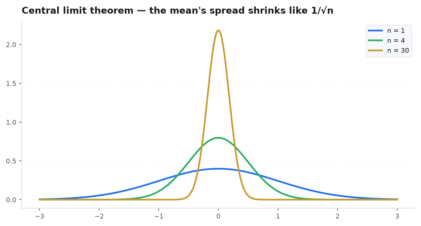
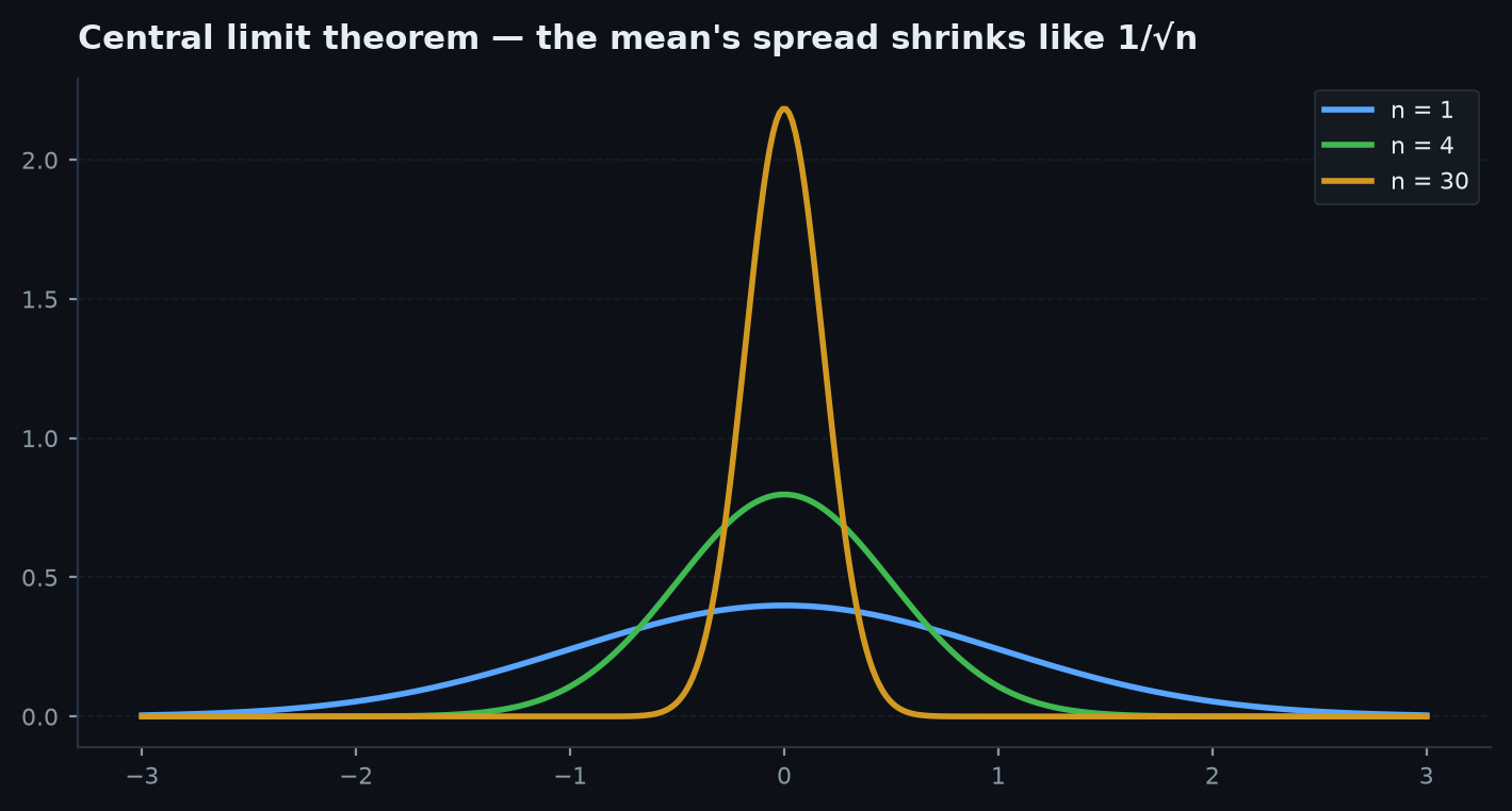
✦Intuition — one flip tells you nothing; a million flips tell you everything

Flip a coin with unknown bias once and you learn almost nothing. Flip it $n$ times and the sample frequency pins the bias down to within about $1/ n$ . That square root is the single most consequential exponent in applied statistics: to halve your uncertainty you must quadruple your data. The LLN is the promise that the estimate converges at all; the CLT is the precise accounting of the residual error — its size and its bell shape. Every backtest t-stat in the gauntlet is these two theorems wearing work clothes.

Modes of convergence#

“ $X_{n} \to X$ ” can mean three different things for random variables, and the two big theorems live at different rungs. Let $X_{1}, X_{2}, \dots$ and $X$ be random variables.

Almost surely (a.s.): $P (lim_{n \to \infty} X_{n} = X) = 1$ — the realised sequence of numbers converges, with probability one. This is the strong law’s mode.
In probability: for every $ε > 0$ , $P (∣ X_{n} - X ∣ > ε) \to 0$ — large deviations become rare, but any single path may misbehave infinitely often. The weak law’s mode.
In distribution: $F_{X_{n}} (x) \to F_{X} (x)$ at every continuity point of $F_{X}$ — only the shapesconverge. The CLT’s mode.

The hierarchy is strict: almost sure $\Rightarrow$ in probability $\Rightarrow$ in distribution, and neither arrow reverses (with one useful exception: convergence in distribution to a constant upgrades to convergence in probability).

✦Two counterexamples worth memorising

In probability but not a.s.: let $X_{n} \sim Bernoulli (1/ n)$ , independent. Then $P (∣ X_{n} ∣ > ε) = 1/ n \to 0$ , so $X_{n} \to 0$ in probability. But $\sum_{n} 1/ n = \infty$ , so by the second Borel–Cantelli lemma $X_{n} = 1$ infinitely often with probability one — the path never settles.

In distribution but not in probability: let $X \sim N (0, 1)$ and $X_{n} = - X$ for all $n$ . Each $X_{n}$ is exactly standard normal, so $X_{n} \to X$ in distribution trivially — yet $∣ X_{n} - X ∣ = 2∣ X ∣$ never shrinks. Distributional convergence says nothing about the variables being close.

The law of large numbers#

Let $X_{1}, X_{2}, \dots$ be i.i.d. with mean $μ$ , and write $X ˉ_{n} = \frac{1}{n} \sum_{i = 1}^{n} X_{i}$ .

WLLN: X ˉ_{n} P μ, SLLN: X ˉ_{n} a.s. μ (needs only E ∣ X_{1} ∣ < \infty) .

✦Proof — WLLN via Chebyshev (assuming finite variance)

Assume $Var (X_{1}) = σ^{2} < \infty$ . By linearity and independence,

E [X ˉ_{n}] = μ, Var (X ˉ_{n}) = \frac{1}{n ^{2}} i = 1 \sum n Var (X_{i}) = \frac{σ ^{2}}{n} .

Chebyshev’s inequality (proved in Inequalities & tail bounds) then gives, for any $ε > 0$ ,

P (∣ X ˉ_{n} - μ ∣ \geq ε) \leq \frac{Var ( X ˉ _{n} )}{ε ^{2}} = \frac{σ ^{2}}{n ε ^{2}} ⟶ 0. ■

The strong law is genuinely harder (Kolmogorov’s proof uses maximal inequalities or backward martingales) and needs only a finite first moment — we state it and move on. The counterexample to keep in mind: the Cauchy distribution has no mean at all, and its sample average never converges — see below.

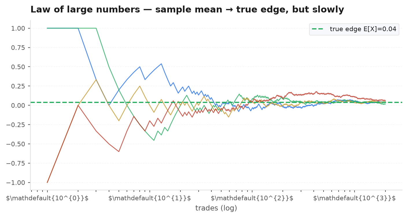
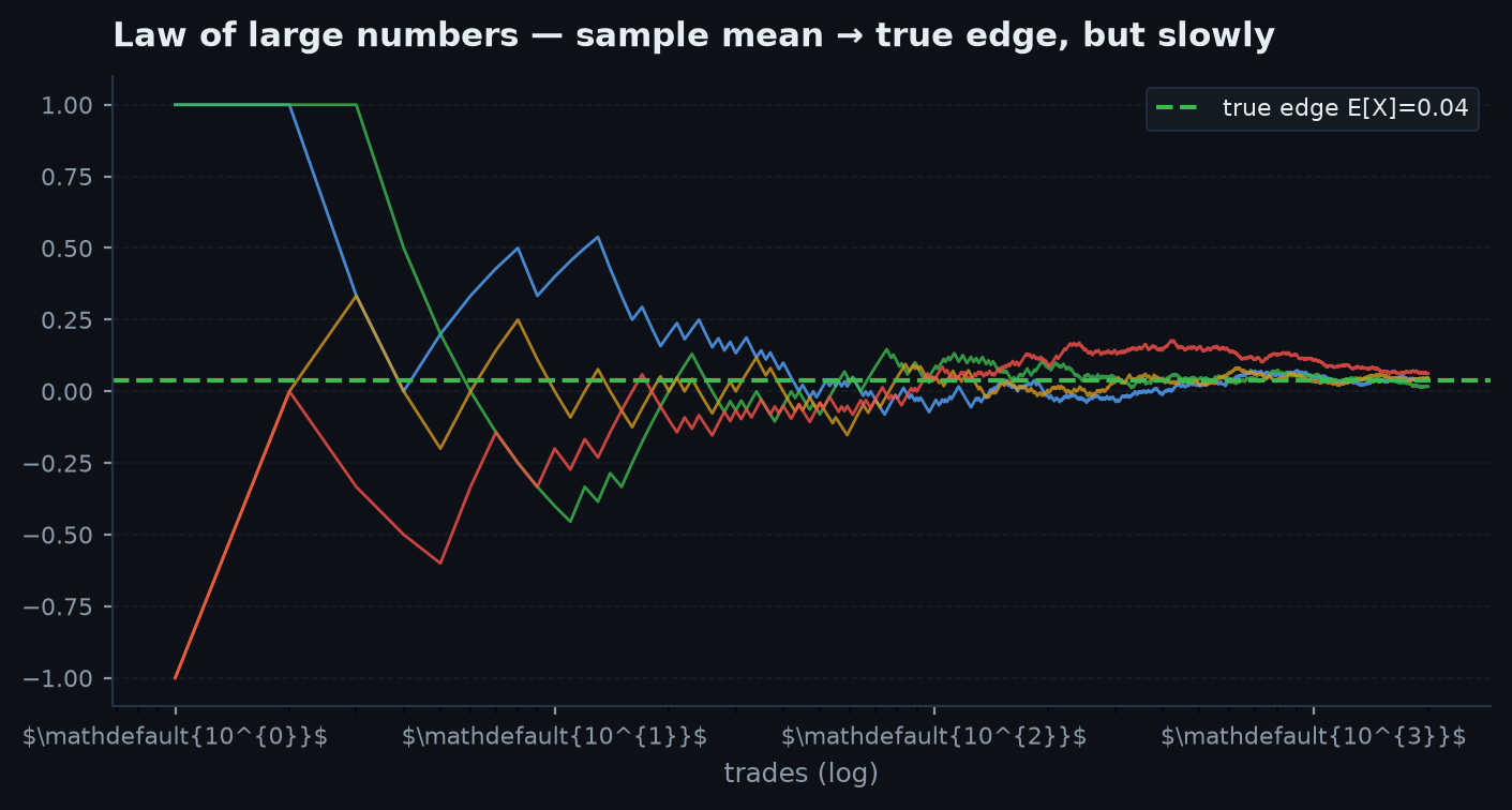
Running sample means of many simulated sequences converging toward the true mean as n grows, with the band of paths narrowing like one over square root of n — The LLN in action: running averages of i.i.d. draws. Early averages are all over the place; by large n every path has been squeezed toward the true mean, with the spread of paths shrinking like 1/sqrt(n) — the rate the CLT will make precise.

Worked example (by hand). A strategy wins $+ 1 R$ with probability $0.55$ and loses $- 1 R$ with probability $0.45$ . Per trade, $μ = 0.10$ and $σ^{2} = E [X^{2}] - μ^{2} = 1 - 0.01 = 0.99$ . How many trades until Chebyshev guarantees $P (∣ X ˉ_{n} - 0.10∣ \geq 0.10) \leq 0.10$ ? Solve $0.99/ (n \cdot 0.01) \leq 0.10$ : $n \geq 990$ . Chebyshev is crude — the CLT will say roughly $n \approx 270$ suffices for the same confidence (solve $1.645 0.99/ n = 0.10$ ) — but the qualitative message stands either way: hundreds of trades, not dozens, before an average is trustworthy.

→Quant lens — why an edge needs hundreds of trades

A per-trade edge of $0.10 R$ against per-trade noise of $\approx 1 R$ is a signal-to-noise ratio of 10:1 against you on every single trade. The LLN is the only thing on your side, and it works at rate $n$ : the t-statistic of the observed mean is roughly $0.10 n$ , so you cross $t = 2$ only near $n = 400$ . A 30-trade backtest of this strategy is statistically silent — which is precisely why backtests lie and why the gauntlet demands sample sizes first.

The central limit theorem#

The LLN says $X ˉ_{n} - μ \to 0$ . The CLT magnifies that vanishing error by $n$ and finds a universal shape.

CLT: if X_{i} i.i.d., E [X_{i}] = μ, Var (X_{i}) = σ^{2} \in (0, \infty), then n \frac{X ˉ _{n} - μ}{σ} d N (0, 1) .

Nothing about the shape of $X_{i}$ survives except its first two moments — skewed, discrete, bimodal, it does not matter, provided the variance is finite. That universality is why the normal distribution is everywhere: it is the unique fixed point of averaging.

✦Proof sketch — CLT via the MGF

Assume the MGF $M (t) = E [e^{tX}]$ exists near 0 (the honest proof uses characteristic functions, which always exist; the algebra is identical). Center and scale: let $Y_{i} = (X_{i} - μ) / σ$ , so $E [Y_{i}] = 0$ , $E [Y_{i}^{2}] = 1$ , and $Z_{n} = \frac{1}{n} \sum Y_{i}$ . By independence,

M_{Z_{n}} (t) = [M_{Y} (t / n)]^{n}, M_{Y} (s) = 1 + = 0 s E [Y] + \frac{s ^{2}}{2} E [Y^{2}] + o (s^{2}) = 1 + \frac{s ^{2}}{2} + o (s^{2}) .

lo g M_{Z_{n}} (t) = n lo g (1 + \frac{t ^{2}}{2 n} + o (\frac{1}{n})) ⟶ \frac{t ^{2}}{2},

which is the MGF of $N (0, 1)$ ; MGF convergence implies convergence in distribution. The whole theorem is Taylor expansion plus $(1 + x / n)^{n} \to e^{x}$ : averaging kills every moment beyond the second at rate faster than $1/ n$ , and only the quadratic term survives. $■$

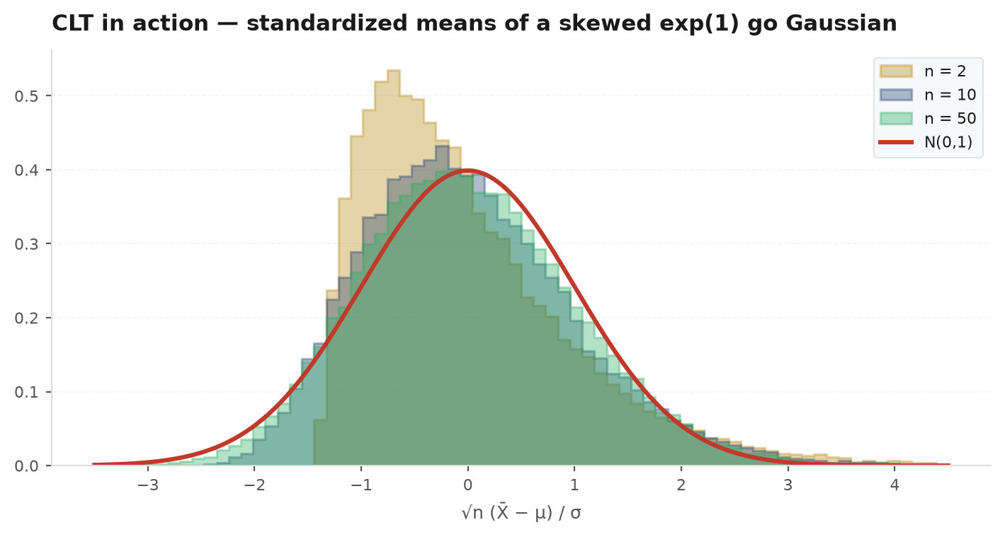
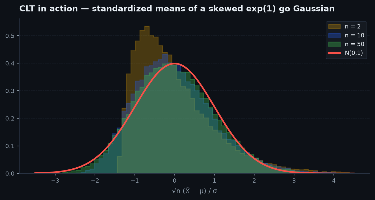
Histograms of standardized sample means of a skewed distribution at increasing sample sizes, morphing from skewed to an almost perfect normal curve — The CLT digesting a skewed distribution. Standardised means of exponential draws: at n = 2 the skew is glaring, at n = 10 it is fading, by n = 50 the histogram is visually indistinguishable from the standard normal overlay. Only mean and variance survive averaging.

How fast is “asymptotic”? The Berry–Esseen theorem gives a uniform, non-asymptotic rate: if $ρ = E ∣ X_{1} - μ ∣^{3} < \infty$ , then

x sup P (Z_{n} \leq x) - Φ (x) \leq \frac{C ρ}{σ ^{3} n}, C \approx 0.4748.

The error decays like $1/ n$ , with the skewness-like ratio $ρ / σ^{3}$ as the constant. Symmetric, thin-tailed summands converge fast (coin flips are excellent by $n = 30$ ); heavily skewed summands — option-selling P&L, for instance — can need thousands of terms before the Gaussian approximation is honest in the tails.

Worked example (by hand). Roll a fair die 100 times; what is $P (S \geq 380)$ ? Per roll $μ = 3.5$ , $σ^{2} = \frac{35}{12} \approx 2.917$ , so $S \approx N (350, 291.7)$ with $sd (S) \approx 17.08$ . Because $S$ is integer-valued, apply the continuity correction: treat ${S \geq 380}$ as ${S > 379.5}$ :

P (S \geq 380) \approx P (Z > \frac{379.5 - 350}{17.08}) = P (Z > 1.727) \approx 4.2%.

Skipping the correction gives $P (Z > 1.756) \approx 4.0%$ — small here, but for coin-flip problems near the mean the half-unit shift is often the difference between a right and a wrong answer.

Sampling distribution of the mean narrowing and becoming Gaussian as the sample size increases — The sampling distribution of the mean: as n grows it both narrows (LLN, width ~ 1/sqrt(n)) and normalises (CLT). Estimation error is not vague — it has a size and a shape, and both are theorems.

The delta method — errors of functions of averages#

Most quantities you report are not averages but functions of averages: a Sharpe ratio, a log growth rate, an implied probability. The delta method pushes the CLT through any smooth function.

✦Derivation — one Taylor step

Suppose $n (θ^_{n} - θ) d N (0, σ^{2})$ and $g$ is differentiable at $θ$ with $g^{'} (θ) \neq = 0$ . Expand: $g (θ^_{n}) = g (θ) + g^{'} (θ) (θ^_{n} - θ) + o_{p} (∣ θ^_{n} - θ ∣)$ . Multiply by $n$ ; the remainder vanishes in probability (Slutsky’s theorem cleans up), leaving

n (g (θ^_{n}) - g (θ)) d N (0, [g^{'} (θ)]^{2} σ^{2}) .

In words: to first order an estimator’s error passes through $g$ scaled by the local slope. Uncertainty is a vector; $g$ stretches it by $∣ g^{'} ∣$ .

Application — the standard error of a Sharpe ratio. With i.i.d. normal-ish returns, the two-dimensional delta method applied to $S R = X ˉ / s$ gives the classic Lo (2002) result

se (S R) \approx \frac{1 + \frac{1}{2} S R ^{2}}{n} .

Plug in numbers: a strategy with true annual Sharpe 1.0 observed over one year of daily data ( $n = 252$ , daily $S R = 1/ 252 \approx 0.063$ ) has daily-scale se $\approx (1 + 0.002) /252 \approx 0.063$ — annualised, $se \approx 1.0$ . One year of daily data measures a Sharpe of 1 to within ±1. The measurement is barely one standard error from zero. The same delta method gives the se of a compound growth rate via $g = lo g$ : relative errors of the mean become absolute errors of the log, which is why log-return standard errors are the clean ones to quote.

When the CLT fails#

Good prep questions push in this direction, and markets live in it. The CLT has three hypotheses — finite variance, independence, identical distribution — and each one fails in a characteristic, tradable way.

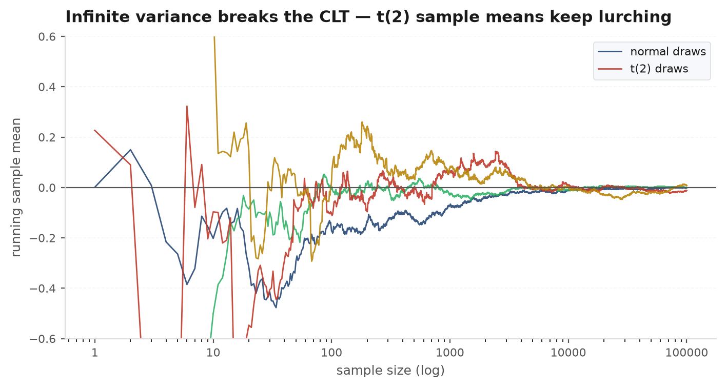
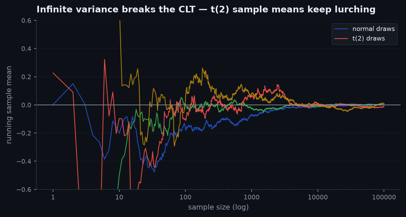
1. Infinite variance — fat tails. If $Var (X) = \infty$ (tail index $α \leq 2$ , e.g. a Cauchy, or a Student-t with 2 or fewer degrees of freedom), sums converge — after different scaling — to stable laws, not the normal. The extreme case is Cauchy: if $X_{i}$ are standard Cauchy, the characteristic function $φ (t) = e^{- ∣ t ∣}$ gives $φ_{X ˉ_{n}} (t) = (e^{- ∣ t ∣/ n})^{n} = e^{- ∣ t ∣}$ — the sample mean of a million Cauchy draws is exactly as spread out as a single draw. Averaging buys you nothing; the LLN itself fails because no mean exists. Real returns are not Cauchy, but their tails are heavy enough ( $α \approx 3$ – $4$ ) that tail probabilities converge to their Gaussian limits punishingly slowly — see the distribution zoo and extreme value theory.

Sample means of t-distributed data with two degrees of freedom failing to tighten into a normal, contrasted with well-behaved data at the same n — CLT failure by fat tails: standardised means of t(2) draws (infinite variance is borderline: variance diverges) keep throwing extreme outliers at every n, while the same experiment on finite-variance data has long since gone Gaussian. When the variance is infinite the bell never forms.

2. Dependence — autocorrelation inflates the variance of the mean. Drop independence but keep stationarity, with autocorrelations $ρ_{k}$ . Expanding the variance of the sum:

Var (X ˉ_{n}) = \frac{1}{n ^{2}} i, j \sum Cov (X_{i}, X_{j}) = \frac{σ ^{2}}{n} (1 + 2 k = 1 \sum n - 1 (1 - \frac{k}{n}) ρ_{k}) \approx \frac{σ ^{2}}{n} (1 + 2 k \geq 1 \sum ρ_{k}) .

A CLT still holds under mixing conditions, but with this inflated variance. Define the effective sample size $n_{eff} = n / (1 + 2 \sum_{k} ρ_{k})$ . For an AR(1) with $ρ_{k} = ρ^{k}$ the factor is $1 + 2 ρ / (1 - ρ)$ : at $ρ = 0.5$ that is 3 — your 1000 correlated observations carry the information of 333 independent ones. Ignore this and every t-stat you compute is inflated by $3$ . Full treatment in time-series statistics.

3. Non-identical terms. Heterogeneous but independent summands still obey a CLT under the Lindeberg (or cruder Lyapunov) condition — no single term may dominate the total variance. The failure mode to remember: a portfolio of 100 tiny positions plus one whale is notGaussian-ised by aggregation; its distribution is the whale’s. Diversification only normalises when risk is genuinely spread.

clt_and_its_failures.py

import numpy as np

rng = np.random.default_rng(11)
reps = 20_000

# 1) CLT works: standardized means of skewed Exponential(1) draws (mu=1, sigma=1)
for n in (2, 10, 50):
    m = rng.exponential(1.0, size=(reps, n)).mean(axis=1)
    z = (m - 1.0) * np.sqrt(n)          # standardized: should be ~ N(0,1) for large n
    # P(Z > 1.645) should approach the Gaussian 5%
    print(f"exp  n={n:3d}  P(Z>1.645) = {(z > 1.645).mean():.4f}   (normal: 0.0500)")

# 2) CLT fails: Cauchy sample means never tighten (no mean, infinite variance)
for n in (10, 1000):
    m = rng.standard_cauchy(size=(reps, n)).mean(axis=1)
    print(f"cauchy n={n:5d}  IQR of sample mean = {np.subtract(*np.percentile(m, [75, 25])):.3f}")
    # IQR is ~2.0 regardless of n: mean of n Cauchys IS a Cauchy

# 3) Dependence: AR(1) with rho=0.5 -> Var(mean) inflated by 1 + 2*rho/(1-rho) = 3
n, rho = 1000, 0.5
eps = rng.normal(0, np.sqrt(1 - rho**2), size=(reps, n))
x = np.zeros((reps, n))
for t in range(1, n):
    x[:, t] = rho * x[:, t - 1] + eps[:, t]      # stationary AR(1), Var(x_t)=1
ratio = x.mean(axis=1).var() / (1.0 / n)          # observed Var(mean) vs iid sigma^2/n
print(f"AR(1) rho=0.5: variance inflation = {ratio:.2f}   (theory: 3.00)")

→Quant lens — the standard error of a backtest, in R and in trades

Take a backtest with mean trade $μ_{R}$ (in R multiples) and per-trade standard deviation $σ_{R} \approx 1$ . The CLT says the observed average is $μ_{R} \pm σ_{R} / n$ , so the t-stat is $t \approx μ_{R} n$ . The sample-size arithmetic every quant should do in their head: detecting an edge of $μ_{R}$ at $t = 2$ needs $n \approx 4/ μ_{R}^{2}$ trades — 400 trades for a $0.1 R$ edge, 10,000 for $0.02 R$ . Then apply the dependence haircut: overlapping positions or clustered signals divide $n$ by the inflation factor above. Most “profitable” backtests die in this paragraph — the theme of hypothesis testing and overfitting detection.

Practice problems#

→Problem 1 — 5,100 heads in 10,000 flips: fair coin?

A coin lands heads 5,100 times in 10,000 flips. Roughly how likely is a deviation this large for a fair coin, and what do you conclude?

Solution. Under fairness, $X \sim Bin (10, 000, 0.5)$ : mean 5,000, standard deviation $10, 000 \times 0.25 = 50$ . So 5,100 heads is exactly $+ 2 σ$ . With continuity correction, $P (X \geq 5100) \approx P (Z > \frac{5099.5 - 5000}{50}) = P (Z > 1.99) \approx 2.3%$ , or $\approx 4.6%$ two-sided. Borderline: a fair coin does this one time in twenty-odd, so it is weak evidence of bias, not proof — exactly the p-value conversation of hypothesis testing. The natural follow-up is “and 51,000 in 100,000?” — now the same 51% rate is $+ 2000/ 25, 000 \approx 6.3 σ$ : the rate deviation matters through $n$ , and what was noise at ten thousand flips is near-certain bias at a hundred thousand.

→Problem 2 — how does the casino always win?

A roulette bet pays even money and wins with probability $18/38$ . The casino takes one million independent $1 bets tonight. Estimate the probability the casino loses money.

Solution. Per bet the casino’s profit has mean $μ = 2/38 \approx 0.0526$ and variance $1 - μ^{2} \approx 0.9972$ , so over $n = 1 0^{6}$ bets total profit is approximately $N (52, 600, 997, 200)$ — standard deviation $\approx 999$ . Losing money means falling $52.6$ standard deviations below the mean: $P (Z < - 52.6)$ , effectively zero ( $\sim 1 0^{- 600}$ ). The lesson to state out loud: the house edge is microscopic per bet but the aggregate is deterministic, because signal grows like $n$ while noise grows like $n$ . A trading firm with a tiny per-trade edge and enough independent trades is this casino — the entire economics of high-frequency trading in one inequality.

→Problem 3 — the Cauchy trap

You average $n$ i.i.d. standard Cauchy random variables. What is the distribution of the sample mean as $n \to \infty$ ?

Solution. It is standard Cauchy for every $n$ — it never converges. Slick proof via characteristic functions: $φ_{X} (t) = e^{- ∣ t ∣}$ , so $φ_{X ˉ_{n}} (t) = [φ_{X} (t / n)]^{n} = (e^{- ∣ t ∣/ n})^{n} = e^{- ∣ t ∣}$ . No contradiction with LLN or CLT: the Cauchy has no mean and infinite variance, so both hypotheses fail. The trap is answering “normal, by the CLT” on reflex. Follow-up worth volunteering: for tails just inside the boundary — t(2), some crypto returns — the CLT technically holds (t(3+)) or fails (t(2)’s variance is infinite), and convergence near the boundary is so slow that pre-asymptotic behaviour, not the limit, is what your risk model actually samples.

→Problem 4 — how many trades to detect a 0.05R edge?

A strategy’s trades have true mean $0.05 R$ and standard deviation $1 R$ . How many trades do you need before the backtest can distinguish it from zero-edge at the 5% level — and with 80% power?

Solution. The t-stat is $t = X ˉ n / σ \approx 0.05 n$ . For bare significance set $0.05 n = 1.96$ : $n \approx (1.96/0.05)^{2} \approx 1, 540$ . But significance if the edge shows up exactly at its mean is a coin flip; for 80% power you need the detection threshold $z_{0.975} + z_{0.80} = 1.96 + 0.84 = 2.80$ standard errors of true edge:

n = (\frac{2.80}{0.05})^{2} = 3, 136 trades.

At 10 trades a week, that is six years of live data. Volunteer the two follow-ons: autocorrelated or overlapping trades shrink $n_{eff}$ and push the number higher still; and if this strategy was the best of $N$ tried, the bar rises again (multiple testing). This one computation is the statistical spine of walk-forward validation.

Next: averages are tamed — now for the extremes. The distribution of the maximum, the k-th largest, records, and why the best-looking of anything is a biased estimate: Order statistics & extremes.