Random walks & Brownian motion

The simple random walk is the fruit fly of probability: simple enough to compute with exactly, rich enough to exhibit recurrence, first passages, reflection symmetry, and the shockingly lopsided arcsine law. Rescale it and it becomes Brownian motion, the continuous backbone of every diffusion model of prices. This chapter derives the walk’s classical results, passes to the limit, and works the barrier-hitting formulas that are really questions about stop-losses in disguise.

✦Intuition — one walk, three questions

Everything here is about a fair coin’s running sum, and three questions about it keep recurring. Does it come back? (Recurrence — yes in 1D, barely; no in 3D.) When does it first reach a level? (First passage — the reflection principle counts the paths.) Where has it spent its time? (The arcsine law — almost never half-and-half.) Each answer transfers verbatim to Brownian motion, where combinatorics is replaced by two martingales, $W_{t}$ and $W_{t}^{2} - t$ , and one symmetry: reflection.

The simple random walk#

Let $ξ_{1}, ξ_{2}, \dots$ be iid with $P (ξ = + 1) = P (ξ = - 1) = \frac{1}{2}$ , and $S_{n} = ξ_{1} + \dots + ξ_{n}$ . Then $E [S_{n}] = 0$ , $Var (S_{n}) = n$ — the $n$ spread — and $S_{n}$ is both a Markov chain (previous chapter) and a martingale (martingales & optional stopping). Exact probabilities are binomial counts: to end at level $k$ after $n$ steps you need $(n + k) /2$ up-steps, so

P (S_{n} = k) = (( n + k ) /2 n) 2^{- n} (n + k even), P (S_{2 n} = 0) = (n 2 n) 2^{- 2 n} \sim \frac{1}{π n},

the asymptotics by Stirling’s formula. Worked example: $P (S_{4} = 0) = (2 4) /16 = 6/16 = 0.375$ , already close to the Stirling estimate $1/ 2 π \approx 0.399$ . That $1/ π n$ decay is slow — and it decides the walk’s fate.

✦Proof sketch — recurrent in 1D and 2D, transient in 3D (Pólya)

Let $m$ be the expected number of visits to the origin. Each return probability contributes an indicator, so $m = \sum_{n} P (S_{n} = 0)$ ; and if the probability of ever returning is $r$ , the number of visits is geometric with mean $1/ (1 - r)$ . Hence: recurrent ( $r = 1$ ) iff the sum diverges. In $d$ dimensions the local CLT gives $P (S_{2 n} = 0) ≍ n^{- d /2}$ (each coordinate must separately return, costing $n^{- 1/2}$ apiece). So the sum behaves like $\sum n^{- d /2}$ : divergent for $d = 1, 2$ (harmonic and worse), convergent for $d \geq 3$ . A drunk man finds his way home; a drunk bird may be lost forever — in 3D the return probability is only about $0.34$ . Note the fine print in 1D: return is certain, but the expected return time is infinite — recurrence without positive recurrence.

The reflection principle#

The walk’s deepest symmetry: fix a level $a > 0$ and let $T_{a} = min {n : S_{n} = a}$ be its first-passage time. Any path that touches $a$ and finishes below it can be reflected about the level $a$ after its first touch, producing an equally likely path finishing the mirrored distance above. Reflection is a bijection on paths, so it is an equality of probabilities:

P (T_{a} \leq n, S_{n} < a) = P (S_{n} > a),

and since ${S_{n} > a} \subset {T_{a} \leq n}$ , adding $P (T_{a} \leq n, S_{n} \geq a)$ to both sides gives the first-passage / running-maximum law with $M_{n} = max_{k \leq n} S_{k}$ :

P (M_{n} \geq a) = P (T_{a} \leq n) = 2 P (S_{n} > a) + P (S_{n} = a) .

A random walk path that touches a barrier level and its mirror image reflected about the barrier after the first touch, illustrating the path bijection — The reflection principle: after the first touch of level a, flip the rest of the path about a. The map is a bijection between paths that touch a and end below it and paths that end above it — so the maximum of the walk has a distribution expressible entirely in terms of the endpoint.

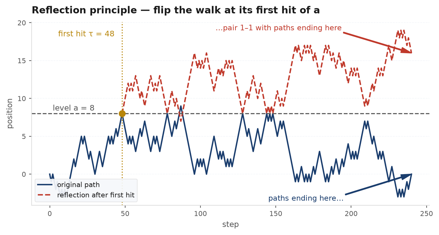
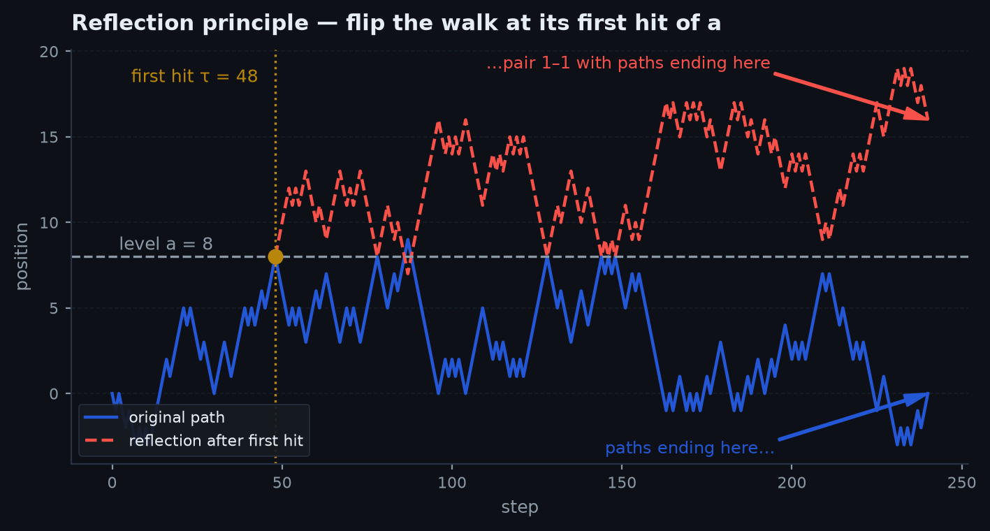
Worked example (by hand). Probability a fair walk reaches $+ 2$ within 4 steps: $P (T_{2} \leq 4) = 2 P (S_{4} > 2) + P (S_{4} = 2) = 2 \cdot \frac{1}{16} + \frac{4}{16} = \frac{6}{16} = 0.375$ . Check directly: hit at step 2 (UU, probability $1/4$ ) or first hit at step 4 (UD UU or DU UU, probability $2/16$ ) — total $6/16$ . The reflection count agrees with brute force.

The same trick proves the ballot theorem, met via martingales in the stopping chapter: if candidate A receives $a$ votes and B receives $b < a$ , the probability A leads throughout the count is $(a - b) / (a + b)$ — reflect the bad paths that touch zero to count them. And for hitting one barrier before another, the martingale route is fastest: for a fair walk (or Brownian motion) started at 0 with barriers $a > 0 > - b$ , optional stopping on $S_{n}$ gives $0 = a p - b (1 - p)$ , so

P (hit a before - b) = \frac{b}{a + b}

— inversely proportional to distance: twice as far means half as likely to be hit first.

Leads and the arcsine law#

Intuition says a fair game spends about half its time in the lead. It does not. Let $L_{n}$ be the number of steps (out of $n$ ) the walk spends positive. The arcsine law says the fraction $L_{n} / n$ converges in distribution to the arcsine distribution:

P (\frac{L _{n}}{n} \leq x) ⟶ \frac{2}{π} arcsin x, density \frac{1}{π x ( 1 - x )},

a U-shaped density: the most likely outcomes are that one side leads nearly the whole time, and the balanced 50/50 split is the least likely. The mechanism is recurrence-in-slow-motion — sign changes require returns to zero, and returns are rare ( $\sim 1/ π n$ ), so the walk gets stuck on one side for long stretches. The same law governs the location of the maximum and the last zero of the path.

→Quant lens — lucky streaks and track records

The arcsine law is the null model of performance streaks. Two strategies flipping the same fair coin will typically show one “dominating” the other for most of a backtest — with zero true edge. A trader up on the year for 10 straight months, a fund ahead of its benchmark since inception: under pure chance these are the typical outcomes, not the surprising ones. Before reading skill into a persistent lead, price in the U-shape — and then run the honest tests in why backtests lie and the multiple-comparison corrections in multiple testing & paradoxes.

arcsine_sim.py

import numpy as np

rng = np.random.default_rng(11)
reps, n = 50_000, 1_000
steps = rng.choice([-1, 1], size=(reps, n))
S = np.cumsum(steps, axis=1)

# fraction of time strictly positive
frac = (S > 0).mean(axis=1)
print((frac <= 0.10).mean())   # ~ (2/pi) arcsin(sqrt(0.1)) = 0.205
print((0.45 <= frac).mean() - (frac > 0.55).mean())
                               # middle decile ~ 0.064 -- rarest region!

# reflection-principle check: P(max of walk >= a) = 2P(S_n > a) + P(S_n = a)
a = 40
print((S.max(axis=1) >= a).mean())                       # empirical
print(2*(S[:, -1] > a).mean() + (S[:, -1] == a).mean())  # reflection formula

From walk to Brownian motion#

Speed the walk up and shrink its steps in the diffusive ratio — $n$ steps per unit time, each of size $1/ n$ — and Donsker’s invariance principle says the whole path

W_{t}^{(n)} = \frac{S _{⌊ n t ⌋}}{n} d W_{t}

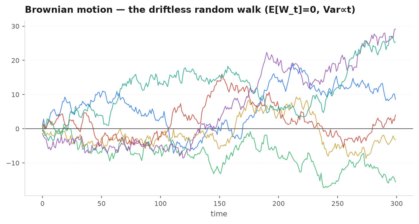
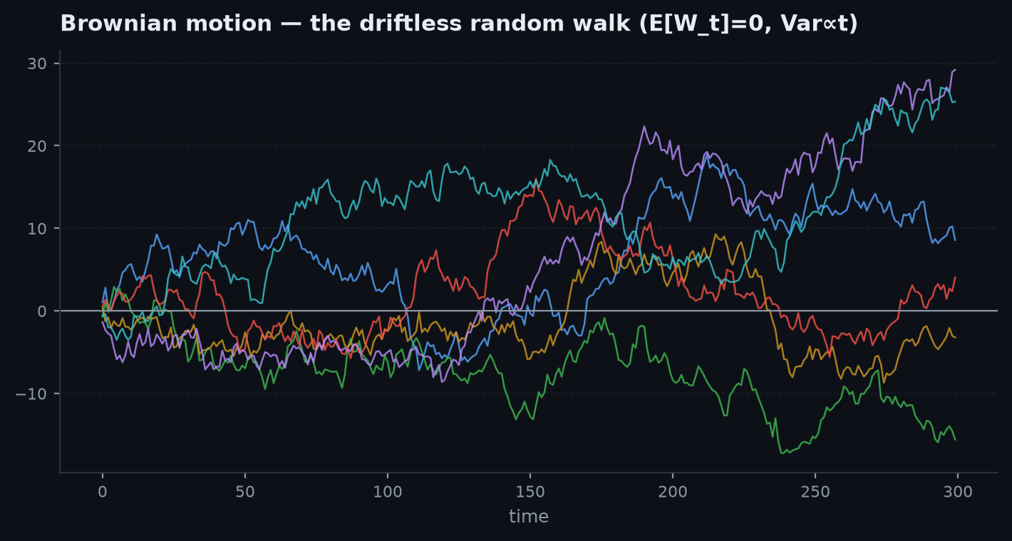
converges to Brownian motion — the CLT (see LLN & CLT) upgraded from a single sum to entire trajectories. Because the limit forgets the step distribution (any finite-variance step works), every path formula proved for the walk by counting — reflection, arcsine, ballot — passes to BM, usually in cleaner form. Recall the definition from the stochastic processes tutorial: $W_{0} = 0$ ; independent increments; $W_{s + t} - W_{s} \sim N (0, t)$ ; continuous paths.

Several sample paths of Brownian motion diverging from zero, with a shaded band widening like the square root of time — Brownian motion: the diffusive limit of the fair random walk. Increments over time t are N(0, t), so the fan of paths widens like sqrt(t) — the continuous version of Var(S_n) = n.

One structural property deserves its own heuristic: quadratic variation. Chop $[0, t]$ into $n$ slices; each squared increment $(Δ W)^{2}$ has mean $t / n$ and variance of order $(t / n)^{2}$ , so the sum of squares has mean $t$ and vanishing variance:

i = 1 \sum n (W_{t_{i}} - W_{t_{i - 1}})^{2} ⟶ t (in probability, as n \to \infty) .

A smooth function has zero quadratic variation; BM has a deterministic, positiveone. This is the precise sense in which “ $(d W)^{2} = d t$ ” holds, the identity that powers Itô’s lemma and the volatility-drag derivation in the tutorial chapter — and it is why realised variance is computed by summing squared returns.

Hitting times and barriers#

Now the barrier toolkit, with barriers $a > 0 > - b$ and $τ = min {t : W_{t} \in {a, - b}}$ . Optional stopping (conditions verified in martingales & optional stopping) applied to the martingale $W_{t}$ gave $P (W_{τ} = a) = b / (a + b)$ above. The second martingale gives the expected exit time.

✦Proof — E[tau] = ab via the martingale W_t^2 − t

$W_{t}^{2} - t$ is a martingale: using independent increments, $E [W_{t + s}^{2} ∣ F_{t}] = E [(W_{t} + (W_{t + s} - W_{t}))^{2} ∣ F_{t}] = W_{t}^{2} + s$ , so subtracting elapsed time restores the fair game. Optional stopping at $τ$ (justified by localisation — stop at $τ \land t$ , use boundedness of $W$ before exit, let $t \to \infty$ ):

0 = E [W_{τ}^{2} - τ] = a^{2} \frac{b}{a + b} + b^{2} \frac{a}{a + b} - E [τ],

E [τ] = \frac{a ^{2} b + a b ^{2}}{a + b} = ab .

The product form is the memorable part: symmetric barriers at $\pm a$ take expected time $a^{2}$ (time scales as distance squared — diffusive scaling again), and widening one barrier lengthens the game only linearly in the other. The identical argument with $S_{n}^{2} - n$ handles the discrete walk, giving $E [τ] = ab$ in steps.

Worked example (by hand). Barriers at $+ 1$ and $- 2$ : hit the near barrier first with probability $2/3$ , and $E [τ] = 1 \times 2 = 2$ time units. In trading dress: a stop 1R below entry and a target 2R above, on a driftless price, is hit-target with probability $1/3$ — the “win rate” of a 2:1 reward-to-risk stop pair is forced to $1/3$ when there is no edge, so payoff asymmetry alone creates nothing. That is the optional stopping theorem talking.

For the one-barrier question — how likely is BM to have touched level $a$ by time $t$ — reflection returns, now as a symmetry of the strong Markov property: a path that touches $a$ before $t$ is equally likely to finish above or below $a$ (the post-touch increment is symmetric). With $M_{t} = max_{s \leq t} W_{s}$ :

P (M_{t} \geq a) = 2 P (W_{t} \geq a) = 2 Φ (- \frac{a}{t}),

with no discrete $P (S_{n} = a)$ correction — continuous paths cannot sit exactly on the barrier at the end with positive probability. Differentiating in $t$ gives the first-passage density of $T_{a}$ (the Lévy distribution, $f_{T_{a}} (t) = \frac{a}{2 π t ^{3}} e^{- a^{2} /2 t}$ ), whose tail is so heavy that $E [T_{a}] = \infty$ : BM hits every level eventually, but the expected wait is infinite — the continuous echo of null recurrence.

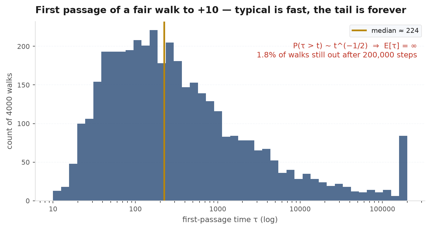
Brownian paths absorbed at an upper barrier with the heavy-tailed first-passage time density and the reflection identity for the running maximum — First passage to a barrier: P(M_t >= a) = 2 P(W_t >= a) by reflection, and the first-passage time has the heavy-tailed Levy density a/sqrt(2 pi t^3) exp(-a^2/2t). Hitting is certain, yet the expected hitting time is infinite.

Drift changes everything. For $X_{t} = μ t + σ W_{t}$ the symmetric martingale is replaced by the exponential martingale $e^{- 2 μ X_{t} / σ^{2}}$ , and optional stopping gives

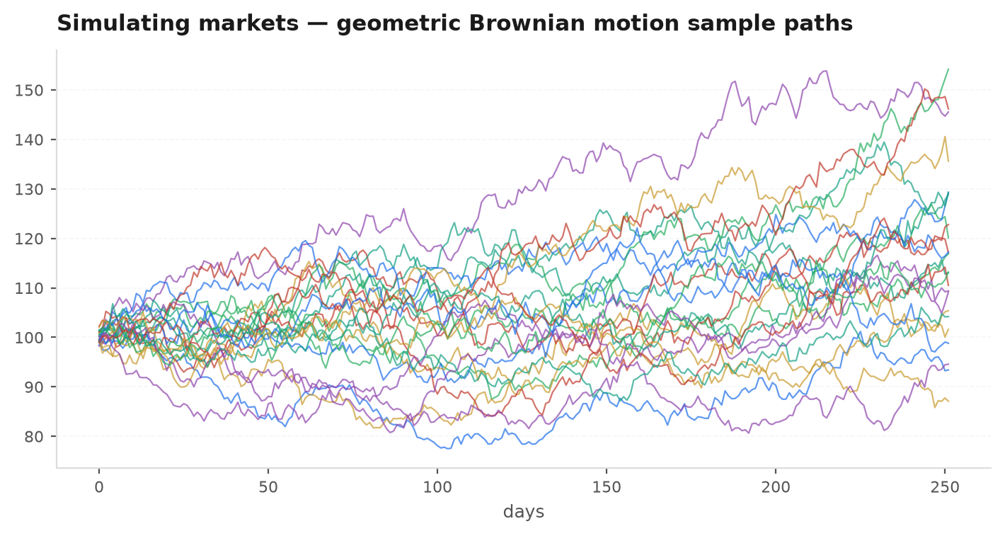
P (hit a before - b) = \frac{e ^{2 μ b / σ^{2}} - 1}{e ^{2 μ b / σ^{2}} - e ^{- 2 μ a / σ^{2}}},

exponentially tilted toward the drift: even a small $μ$ dominates the barrier odds over long horizons, because drift grows like $t$ while noise grows like $t$ . With zero variance the process is a deterministic line and hits only the barrier on the drift’s side — the formula’s $σ \to 0$ limit. These barrier identities price knock-outs, model stop-loss survival, and underlie drawdown mathematics on the simulated GBM paths shown below.

Many simulated geometric Brownian motion price paths starting from one point, fanning out into a right-skewed log-normal cloud, with the mean path above the median path — Geometric Brownian motion — exp of a drifted BM — is where these hitting results earn money: barrier-option knock-out probabilities, stop-loss survival curves, and drawdown distributions are all first-passage calculations on the log-price.

Practice problems#

→Problem 1 — Does the walk return to zero?

A fair simple random walk starts at 0. What is the probability it eventually returns to 0? What about the walk on $Z^{3}$ ?

Solution. Let $r$ be the return probability. The number of visits to 0 is geometric with mean $1/ (1 - r)$ , but that mean also equals $\sum_{n} P (S_{n} = 0) \approx \sum_{n} \frac{1}{π n} = \infty$ — so $1/ (1 - r)$ is infinite and $r = 1$ : the 1D walk is recurrent. The follow-up trap: the expected return time is infinite (the return-time distribution has a $n^{- 3/2}$ tail), so “it always comes back” and “on average it never comes back” are simultaneously true. In 3D the return probabilities decay like $n^{- 3/2}$ , the sum converges, and the return probability drops to $\approx 0.34$ — transience. Mean-reversion claims for a market price are claims about which regime it is in; recurrence of a fair walk is not an edge, because the wait is unbudgetable.

→Problem 2 — Expected time to exit [−a, a]

A fair simple random walk starts at 0. Find the expected number of steps until $∣ S_{n} ∣ = a$ .

Solution. $S_{n}^{2} - n$ is a martingale: $E [S_{n + 1}^{2} ∣ F_{n}] = S_{n}^{2} + 2 S_{n} E [ξ] + 1 = S_{n}^{2} + 1$ . Optional stopping at the exit time $τ$ (bounded increments, and $E [τ] < \infty$ since exit happens with positive probability in each block of $2 a$ steps): $E [S_{τ}^{2}] - E [τ] = 0$ . But $S_{τ}^{2} = a^{2}$ always, so $E [τ] = a^{2}$ . First-step analysis from the Markov chapter confirms it: solving $k_{i} = 1 + \frac{1}{2} k_{i - 1} + \frac{1}{2} k_{i + 1}$ with $k_{\pm a} = 0$ gives $k_{i} = a^{2} - i^{2}$ . Diffusive scaling in one line: doubling the range quadruples the time. For asymmetric barriers $a, b$ the same argument yields $ab$ .

→Problem 3 — P(BM hits 1 before −2)

Standard Brownian motion starts at 0. What is the probability it reaches $+ 1$ before $- 2$ ? And the expected time until it hits one of them?

Solution. Stop the martingale $W_{t}$ at the two-barrier exit $τ$ . With $p = P (hit 1 first)$ : $0 = E [W_{τ}] = 1 \cdot p + (- 2) (1 - p)$ , so $p = 2/3$ — the general $b / (a + b)$ with $a = 1, b = 2$ . Then $W_{t}^{2} - t$ gives $E [τ] = ab = 2$ . Sanity checks worth running: the answer depends only on the barrier ratio (BM is scale-invariant: $c^{- 1} W_{c^{2} t}$ is again BM), and as $b \to \infty$ , $p \to 1$ — with the lower barrier removed, recurrence guarantees hitting $+ 1$ eventually, though (Problem 1’s moral) in infinite expected time.

→Problem 4 — Distribution of the maximum of BM

Find the distribution of $M_{t} = max_{s \leq t} W_{s}$ , and compute $P (M_{1} \geq 1)$ and $E [M_{t}]$ .

Solution. By reflection at the first touch of $a$ (strong Markov + symmetry): $P (M_{t} \geq a) = 2 P (W_{t} \geq a) = 2Φ (- a / t)$ . Equivalently $M_{t} = d ∣ W_{t} ∣$ — the running maximum has the same law as the absolute endpoint, a genuinely surprising identity. Numbers: $P (M_{1} \geq 1) = 2Φ (- 1) \approx 0.317$ , double the endpoint probability $Φ (- 1) \approx 0.159$ . And $E [M_{t}] = E ∣ W_{t} ∣ = 2 t / π \approx 0.798 t$ (the folded-normal mean from the zoo). Quant reading: over any horizon, the expected high-water mark of a driftless account is about $0.8 σ t$ — noise alone manufactures impressive-looking peaks, which is the correct null when admiring an equity curve’s best point.

→Problem 5 — How long is the lead?

Two people flip a fair coin 1,000 times; A scores on heads, B on tails. Which is more likely: the running score is tied in share of time-in-lead (each leads about 50%), or one player leads more than 90% of the time?

Solution. The lopsided outcome wins, and it is not close. By the arcsine law the fraction of time A leads has density $1/ (π x (1 - x))$ , minimised at $x = 1/2$ and blowing up at the edges. Quantitatively,

P (one side leads > 90%) = 2 (1 - \frac{2}{π} arcsin 0.9) \approx 0.41,

while $P (0.45 \leq share \leq 0.55) = \frac{2}{π} (arcsin 0.55 - arcsin 0.45) \approx 0.064$ . A 9-to-1 domination is six times likelier than a near-even split. The mechanism to narrate: leads change only at zeros of the walk, zeros arrive at rate $\sim 1/ n$ , so a 1,000-flip game has only ~25 expected ties — the lead is sticky. This is the standard counter-question to “my strategy has beaten the benchmark almost all year”: under the no-edge null, that is the modal outcome, not evidence.

Next: the tools are assembled — counting, conditioning, indicators, martingales, walks. Now the victory lap: the classic brainteasers of the quant canon, each solved fast and solved rigorously. Probability brainteasers.