Stochastic processes

A price path is a single draw from a random process. To reason about it — to simulate it, to price risk against it, to know what “no edge” looks like — you need the mathematics of random motion: random walks, martingales, Brownian motion, and the geometric Brownian motion that underlies almost every model of asset prices. This chapter builds them in order, states Itô’s lemma, and uses it to re-derive the volatility drag you first met in Part II — this time from the calculus of randomness.

✦Intuition — why a trader learns this at all

You only ever see one price path — the one that happened. But to judge a strategy you need to ask what could have happened: was that $+ 30%$ year skill, or one lucky draw from a process that just as easily hands you $- 20%$ ? To answer that you need a model of the coin the market is flipping. This chapter builds that model in three steps — a fair coin-flip walk (the “no edge” null), its smooth continuous-time limit (Brownian motion), and the version that keeps prices positive and compounding (geometric Brownian motion). The payoff is concrete: it tells you what random looks like (so you can spot when your backtest isn’t), and it explains — from calculus, not hand-waving — why a volatile asset compounds slower than its average return suggests.

Random walks and martingales#

Start discrete. A random walk is a running sum of independent shocks $ξ_{t}$ :

P_{t} = P_{t - 1} + ξ_{t}, E [ξ_{t}] = 0, the ξ_{t} independent .

Its defining property is that the best forecast of tomorrow, given everything you know today (the information set $F_{t}$ ), is simply today’s value. A process with that property is a martingale:

E [P_{t + 1} ∣ F_{t}] = P_{t} ⟺ E [next return ∣ past] = 0.

The martingale is the mathematical statement of no edge. If prices are a martingale, no rule built from past information can produce positive expected return — a theorem (the optional-stopping theorem) that no stop, target, or entry timing can beat. This is why the martingale is the null hypothesis the whole gauntlet tests against: an edge is precisely a departure from the martingale property, a conditional expectation that drifts up rather than staying flat.

→Efficient markets, restated

The weak-form efficient-market hypothesis is just the claim that prices are (close to) a martingale with respect to past prices. Every technical strategy is, mathematically, a bet that this claim is false for some conditioning information. Most of the time, on most instruments, it is very nearly true — which is why edges are small, rare, and quick to decay.

Brownian motion#

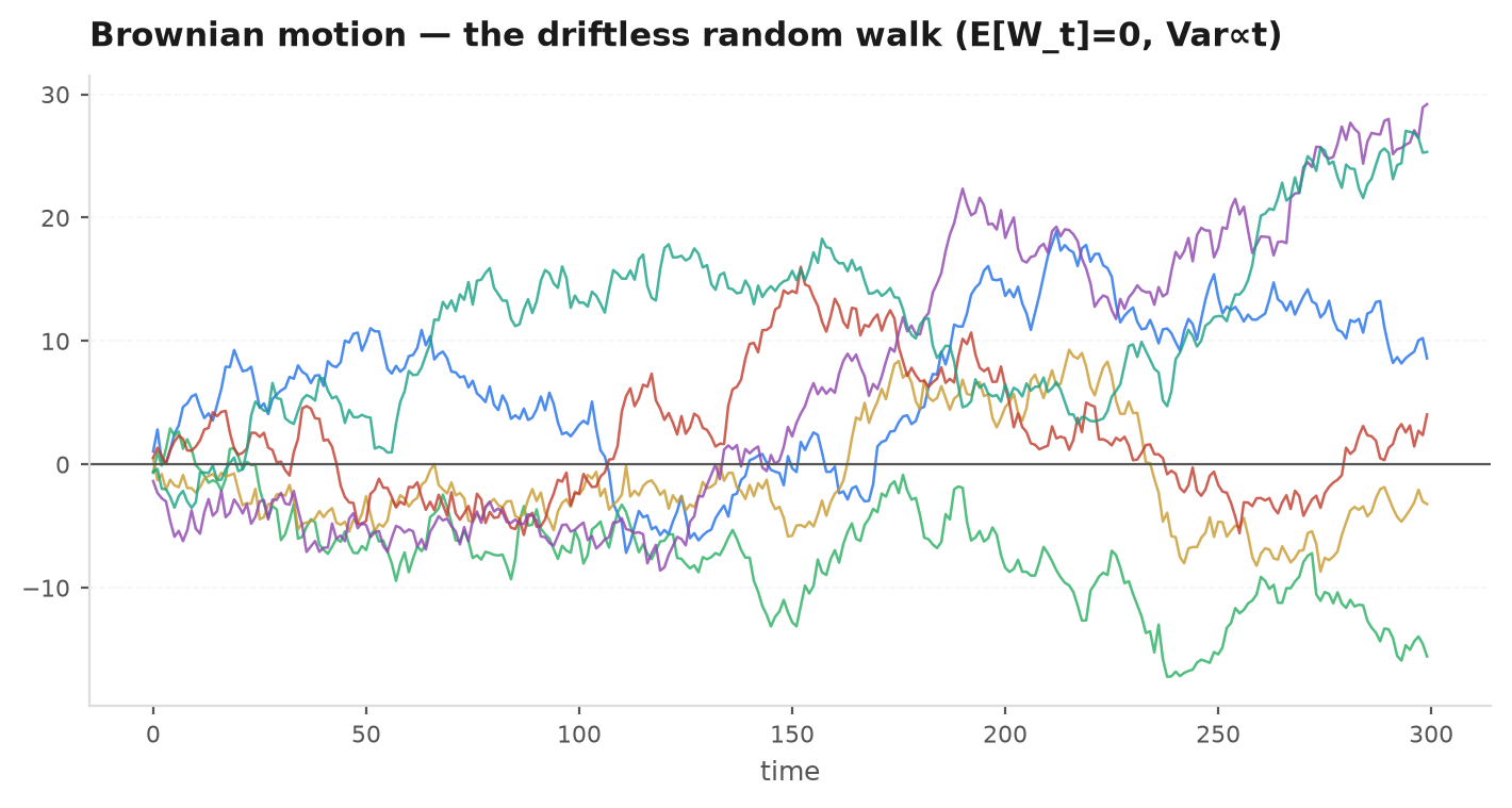
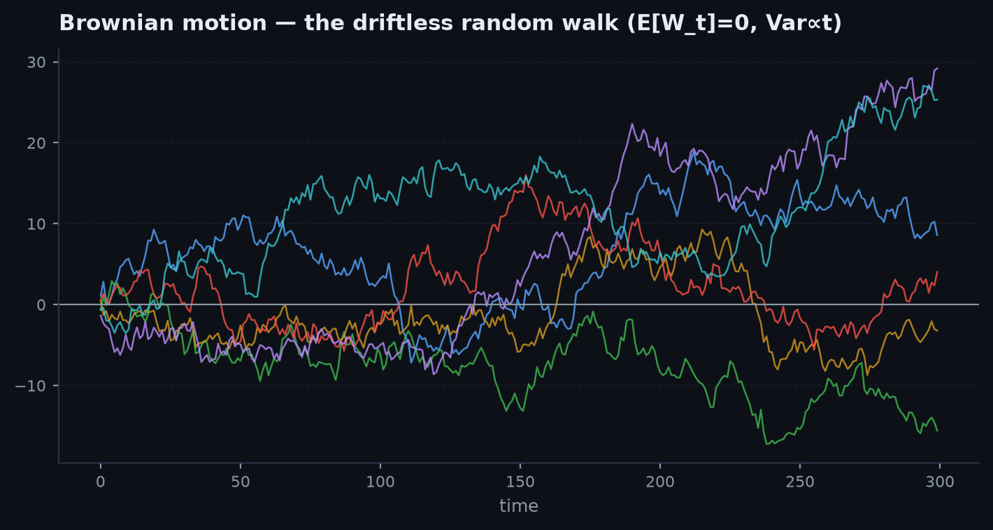
Take the random walk to a continuous-time limit — shrink the step size and let steps arrive infinitely often — and it converges (by the central limit theorem) to Brownian motion $W_{t}$ , also called the Wiener process. It is defined by four properties:

Starts at zero: $W_{0} = 0$ .
Independent increments: non-overlapping changes are independent — the future is uncorrelated with the past given the present (the continuous-time martingale property).
Gaussian increments: over an interval of length $t$ , the change is normal with variance equal to the elapsed time, $W_{s + t} - W_{s} \sim N (0, t)$ .
Continuous paths (but nowhere differentiable — the path is infinitely jagged).

The variance-proportional-to-time property is the one to hold onto: $Var (W_{t}) = t$ , so the standard deviation grows like $t$ . This is the famous square-root-of-time scaling: risk over a horizon grows with its square root, not linearly. It is the same $n$ that governs the standard error of a measured edge — dispersion accumulates like the root of the number of independent increments.

Several sample paths of Brownian motion diverging from zero, with a shaded band widening like the square root of time — Sample paths of Brownian motion. Each jagged line is one realisation; they fan out from the origin, and the spread grows like sqrt(t) (the shaded band). No path is differentiable — the increments are pure independent Gaussian noise, the continuous limit of a fair coin-flip walk.

✦The key scaling rule for increments

Over a small time step

d t

, the Brownian increment

d W

has mean zero and variance

d t

— so informally

d W \sim d t N (0, 1)

and, crucially,

(d W)^{2} \to d t

. That last identity looks strange but is the engine of Itô’s lemma below: the square of a random increment is not negligible next to

d t

— it is

d t

Geometric Brownian motion#

Prices cannot be modelled as plain Brownian motion — that would let them go negative, and a $10 move should mean something different for a $20 stock than a $2000 one. The fix is to make the proportional change follow Brownian motion. That is geometric Brownian motion (GBM), written as a stochastic differential equation:

d S = μ S d t + σ S d W .

The first term is a deterministic drift at rate $μ$ ; the second is random diffusion with volatility $σ$ . Both scale with $S$ , so returns — not dollar moves — are what is stationary. This is the model behind Black-Scholes and behind the Monte-Carlo engine in Simulating markets.

Itô’s lemma and the solution#

To solve the SDE we need the chain rule for stochastic processes, which is not the ordinary one. Itô’s lemma says: for a smooth function $f (S)$ of a process driven by $d S = a d t + b d W$ ,

df = (\frac{\partial f}{\partial t} + a \frac{\partial f}{\partial S} + \frac{1}{2} b^{2} \frac{\partial ^{2} f}{\partial S ^{2}}) d t + b \frac{\partial f}{\partial S} d W .

The extra term — the second-derivative piece — is what distinguishes Itô calculus from ordinary calculus. It appears because $(d W)^{2} = d t$ is first-order, not second-order, so a Taylor expansion must keep the quadratic term. Apply it to $f = ln S$ to solve GBM.

✦Derivation — apply Itô to ln S, get the −σ²/2 drift

For GBM, $a = μ S$ and $b = σ S$ . With $f (S) = ln S$ the derivatives are $\partial f / \partial S = 1/ S$ and $\partial^{2} f / \partial S^{2} = - 1/ S^{2}$ (no explicit time dependence). Substitute:

d (ln S) = (μ S \cdot \frac{1}{S} + \frac{1}{2} σ^{2} S^{2} \cdot (- \frac{1}{S ^{2}})) d t + σ S \cdot \frac{1}{S} d W .

d (ln S) = (μ - \frac{1}{2} σ^{2}) d t + σ d W .

Now $ln S$ follows a plain Brownian motion with constant drift, so it integrates trivially: $ln S_{t} - ln S_{0} = (μ - \frac{1}{2} σ^{2}) t + σ W_{t}$ . Exponentiate to get the closed-form solution of GBM:

S_{t} = S_{0} exp [(μ - \frac{1}{2} σ^{2}) t + σ W_{t}] .

Why it matters: the growth rate of the logarithm — the compound rate you actually earn — is $μ - \frac{1}{2} σ^{2}$ , not $μ$ . The $- \frac{1}{2} σ^{2}$ is volatility drag, and here it drops out of Itô’s lemma automatically: the concavity of $ln$ (its negative second derivative) turns variance into a systematic penalty on compound growth. Two assets with the same arithmetic drift $μ$ but different volatility compound at different rates — the more volatile one lags by exactly half its variance.

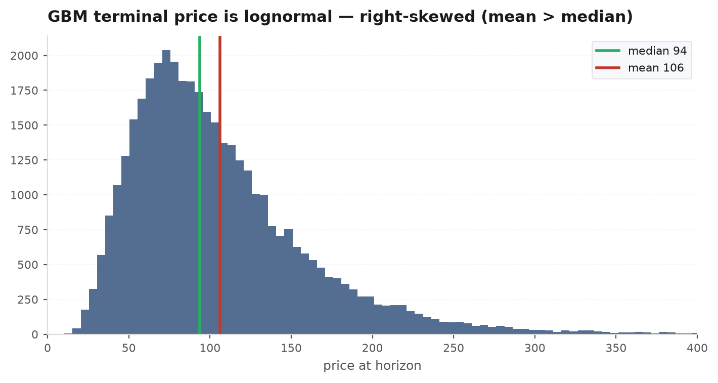
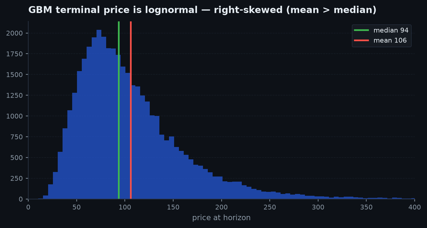
Because $ln S_{t}$ is normal, $S_{t}$ is log-normal — positive, right-skewed, and with a median ( $S_{0} e^{(μ - σ^{2} /2) t}$ ) that sits below its mean ( $S_{0} e^{μ t}$ ). The typical path underperforms the average path; a few big winners drag the mean above the median. That gap is the drag, made visual.

A right-skewed histogram of the terminal price of a geometric Brownian motion, with the median marked to the left of the higher mean — The terminal price of a GBM is log-normal — the distribution of where the paths end up. It is right-skewed: most outcomes bunch below, a thin tail of big winners pulls the mean to the right of the median. That mean-above-median gap is exactly the volatility drag the −sigma^2/2 term encodes.

✦Scenario — the drag on a calm index vs a wild altcoin, over one year

Two instruments, one year ( $t = 1$ ). A broad equity index with arithmetic drift $μ = 10%$ and volatility $σ = 20%$ ; and an altcoin with a fat $μ = 30%$ drift but $σ = 80%$ volatility. Itô says the compound growth rate is $μ - \frac{1}{2} σ^{2}$ , so plug in the numbers:

index: 0.10 - \frac{1}{2} (0.20)^{2} = 0.08, altcoin: 0.30 - \frac{1}{2} (0.80)^{2} = - 0.02.

The index compounds at $8%$ — the $2%$ drag is a mild tax. The altcoin is the shock: despite a $+ 30%$ average return, its $32%$ drag makes the median holder lose money — the typical one-year path ends at $S_{0} e^{- 0.02} = 0.98 S_{0}$ , down $2%$ , while the mean ends at $S_{0} e^{0.30} = 1.35 S_{0}$ , up $35%$ . The gap between them is not a paradox: a handful of moon-shot paths haul the average up while most paths quietly bleed. At the desk this is why you size on log growth, not headline drift, and why leverage on a high-vol asset can have a negative expected compound rate even when each bet has positive expected return — the same volatility drag you met in returns and compounding, now falling straight out of the second-derivative term in Itô’s lemma.

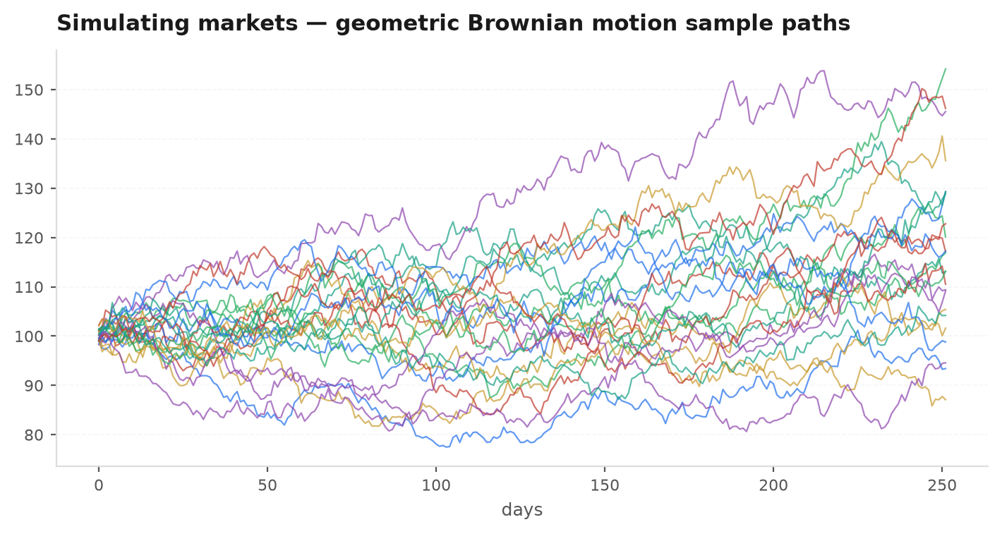
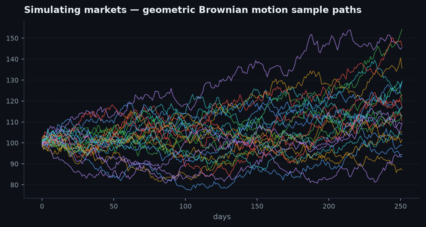
Many simulated geometric Brownian motion price paths starting from one point, fanning out into a right-skewed log-normal cloud, with the mean path above the median path — Simulated GBM price paths. They start at one price and fan into a right-skewed cloud: most paths cluster low while a few run away high, so the mean path (upper line) sits above the median path (lower line). The wedge between them is volatility drag — the reason median wealth grows at mu − sigma^2/2, not mu.

gbm_sim.py

import numpy as np

# One GBM path via the exact log-solution (no discretisation error):
#   S_t = S_0 * exp((mu - sigma^2/2) t + sigma W_t)
S0, mu, sigma, T, steps = 100.0, 0.08, 0.20, 1.0, 252
dt = T / steps
dW = np.random.normal(0.0, np.sqrt(dt), steps)      # increments ~ N(0, dt)
logS = np.log(S0) + np.cumsum((mu - 0.5*sigma**2)*dt + sigma*dW)
path = np.exp(logS)                                  # a single log-normal price path

Why model prices this way — and where it breaks#

GBM earns its place because it captures the three things that matter most cheaply: prices stay positive, returns compound multiplicatively, and volatility scales with the square root of time. It gives closed-form option prices and trivially fast simulation. But it is a model, and its assumptions are exactly where real markets bite back:

GBM assumes	Reality	Consequence
Gaussian log-returns	Fat tails — extreme moves far more likely	Underestimates crash / gap risk
Constant volatility σ	Volatility clusters and spikes (GARCH-like)	Mis-prices risk in regime shifts
Continuous paths	Prices jump (gaps, halts, news)	Stops slip; no continuous hedging
Independent increments	Short-horizon autocorrelation, trends	The very thing edges exploit

!The thin tails are the dangerous lie

The single most consequential flaw is the Gaussian assumption. Real return distributions are leptokurtic— the tails are far heavier than the normal, so “20-sigma” days that a Gaussian says happen once in the age of the universe actually happen every few years. A risk model built on pure GBM will systematically under-reserve for the moves that blow up accounts. This is why edgekit’s risk tools report empirical tail statistics (VaR/CVaR from resampled real returns) rather than trusting a fitted normal, and why the last independent-increment row is, ironically, the one an edge is a bet against.

The right stance is instrumental: GBM is the frictionless baseline you reason from, the “no edge, no fat tails” null. Simulation lets you keep its convenience while swapping in fatter tails and clustered volatility to stress-test what the closed form hides.

Next: these processes are exactly what a Monte-Carlo engine draws from — and how you generate thousands of plausible futures to stress a strategy. Simulating markets.