Time-series statistics
Everything in classical statistics quietly assumed independent observations. Financial data laugh at that: returns cluster, prices trend, volatility begets volatility. This chapter rebuilds the essentials for dependent data — stationarity, autocovariance, white noise versus iid — works the AR(1) model completely (mean, variance, ACF, the unit root at ), derives how autocorrelation shrinks your effective sample size, and demonstrates the spurious-regression trap that has fooled a century of researchers.
With iid data, 1,000 observations carry 1,000 observations’ worth of information. With positively autocorrelated data, consecutive points partly repeat each other — you may effectively have 300, and every standard error computed under the iid assumption is too small, every t-statistic too large, every backtest too confident. Worse, if the series is not even stationary — if its mean or variance drifts — then averaging over time estimates nothing at all: there is no fixed quantity to converge to. The two questions of this chapter, in order: is there a stable distribution to learn about? (stationarity), and how fast do we learn it? (autocorrelation and effective sample size).
Stationarity: strict and weak#
A process is strictly stationary if every finite-dimensional distribution is shift-invariant: for all and time points. It is weakly (covariance) stationary if only the first two moments are shift-invariant:
Neither implies the other in general. Strict + finite second moments weak; but an iid sequence of Cauchy variables is strictly stationary and not weakly stationary (no variance exists — see the distribution zoo). Conversely a weakly stationary process can have wildly time-varying higher moments. Counterexamples to hold in mind:
- White noise: stationary (both senses if iid Gaussian). The boring baseline.
- Random walk : not stationary in any sense — grows without bound. Its increments are stationary.
- Deterministic seasonality : the mean depends on — not stationary, though it looks tame.
- GARCH returns: weakly stationary (constant unconditional moments) yet the conditional variance moves every day — stationarity is about unconditional distributions.
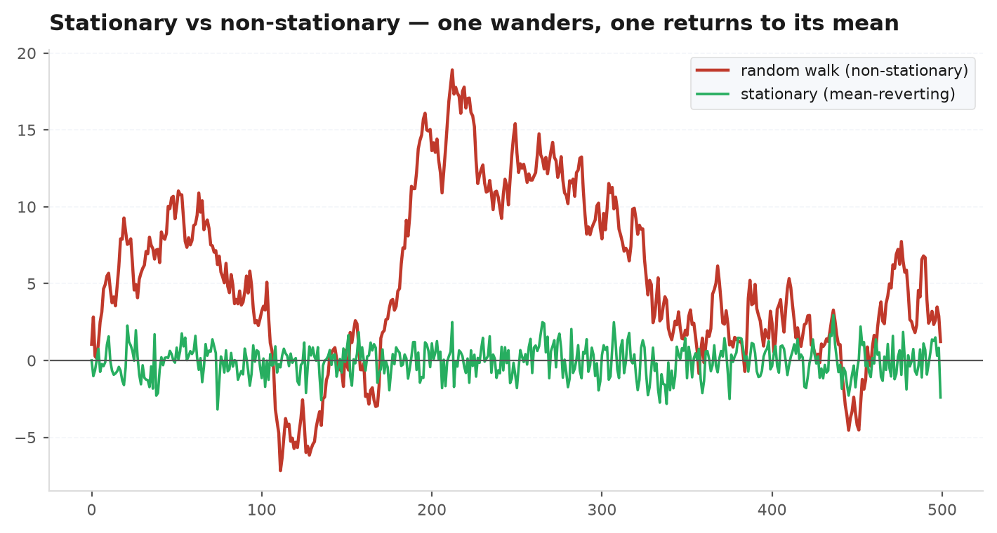
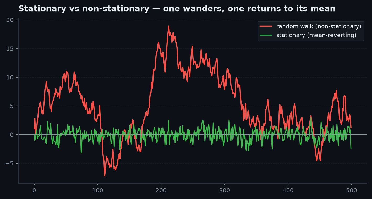
Autocovariance, autocorrelation, and white noise vs iid#
For a weakly stationary process, define the autocovariance and autocorrelation . Basic properties: (symmetry), (Cauchy–Schwarz, proved in Inequalities & tail bounds), and the whole function must be positive semi-definite — because for any weights, exactly the argument that makes covariance matrices PSD in Joint distributions. Not every damped sequence is a valid ACF.
White noise means mean zero, constant variance, and for — uncorrelated, nothing more. IID is strictly stronger: independence kills all functional relationships, not just linear ones. The canonical finance example of the gap: GARCH returns are white noise (uncorrelated — no linear predictability, consistent with a martingale null) while their squares are strongly autocorrelated — volatility is predictable even when direction is not. This ARCH effect is the single most robust stylised fact of asset returns, and the reason ARIMA & GARCH is a chapter and not a footnote.
AR(1), worked completely#
The workhorse model of mean reversion. With :
Stationary solution. Iterate the recursion backwards times:
If , the term (in mean square) and the sums converge, leaving the MA(∞) representation — a fixed, time-invariant filter of the noise, hence stationary. If no stationary solution exists.
Mean. Take expectations of the recursion under stationarity ( ): .
Variance. Because is uncorrelated with (which depends only on older noise), variances add:
ACF. Multiply the (centred) recursion by , , and take expectations; the noise term drops out:
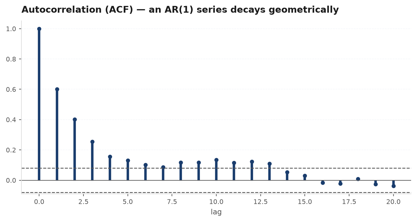
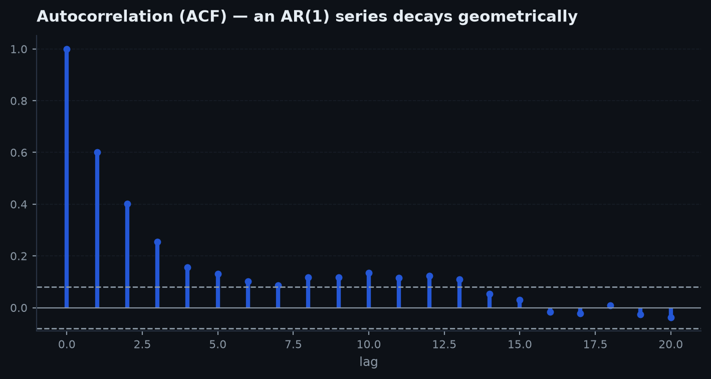
Geometric decay with rate — the process forgets its past exponentially, with half-life . These Yule–Walker steps are the derivation to be able to do on a whiteboard.
Worked numbers. Daily spread with . Long-run mean ; stationary variance , sd — more than double the shock sd, because shocks accumulate before decaying. Autocorrelations: ; half-life days — the timescale a mean-reversion trade on this spread should hold for.
The unit root. At (and ) the recursion is the random walk: , with and : shocks are permanent, nothing mean-reverts, and every formula above (mean , variance ) divides by zero. The boundary between (stationary, slow) and (nonstationary) is statistically delicate but conceptually absolute — it is the difference between a spread you can trade back to fair value and one that has no fair value.
MA(1) and the AR/MA signatures#
The moving-average counterpart: . Mean ; variance ; first autocovariance (only the shared shock overlaps); and for — the ACF cuts off dead after lag 1:
That bound is a classic result in itself: no MA(1) can have first-lag autocorrelation above one half (maximise by calculus, or note ). The identification signatures, read off any pair of ACF/PACF plots:
| Model | ACF | PACF (partial ACF) |
|---|---|---|
| AR(p) | Geometric / oscillating decay | Cuts off after lag p |
| MA(q) | Cuts off after lag q | Geometric decay |
| ARMA(p,q) | Decay after lag q | Decay after lag p |
| White noise | Zero at all lags (within ±1.96/√n bands) | Zero at all lags |
Autocorrelation and the sample mean: effective sample size#
Now the practical payoff. For a stationary series, the variance of the sample mean is not :
Expand the variance of the sum and collect by lag (there are pairs at lag ):
For AR(1), , so the inflation factor is
At the factor is 3: a thousand autocorrelated observations estimate the mean as precisely as 333 independent ones, and iid-based standard errors are too small by — enough to turn a t-statistic of 2.0 into an honest 1.15. This is the same correction the CLT chapter derived (LLN & the CLT), the reason Newey–West/HAC standard errors exist in regression, and the reason the block bootstrap resamples blocks.
Spurious regression#
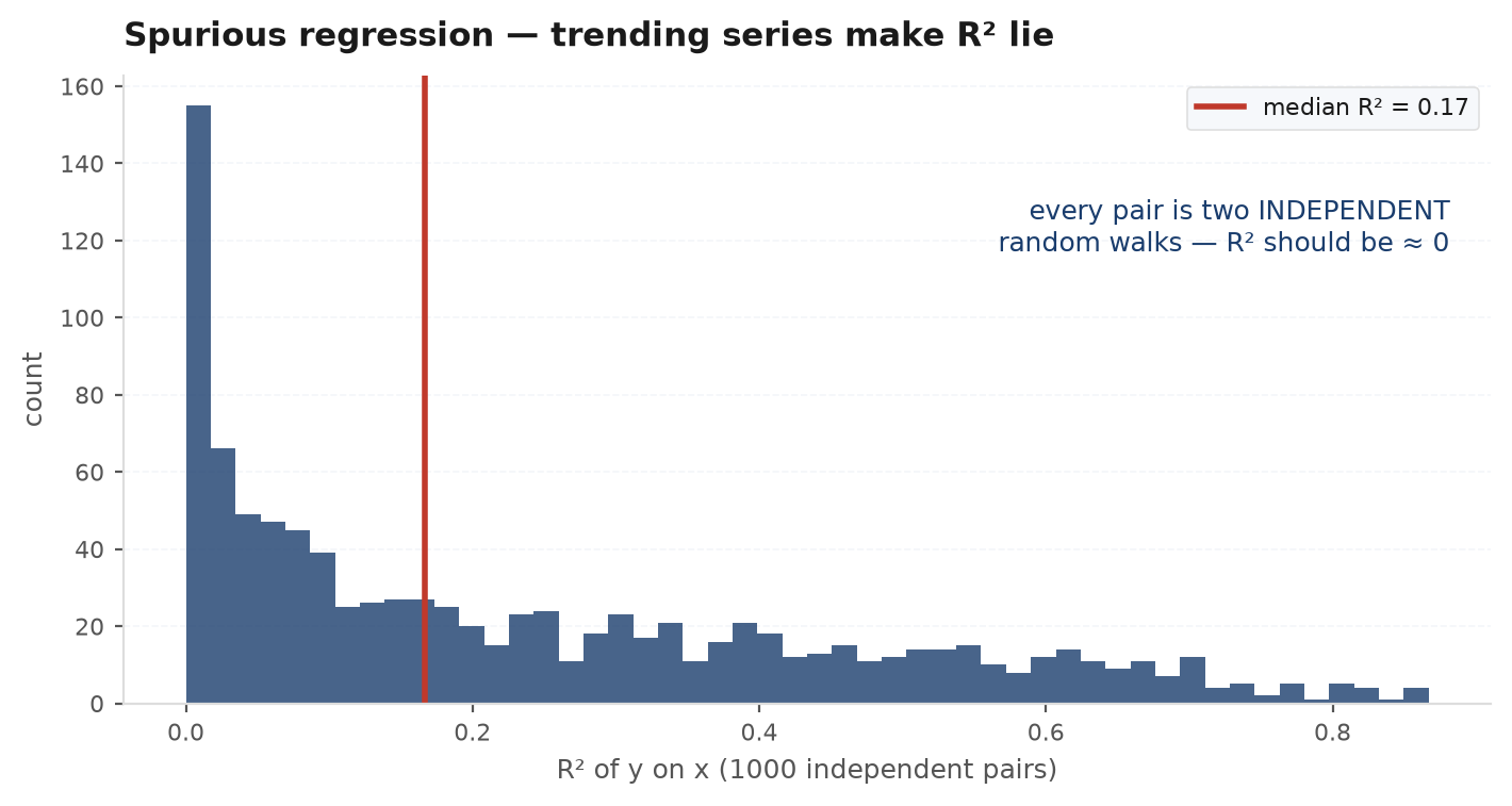
The most expensive mistake in applied time series: regress one trending series on another, unrelated one, and the regression looks superb. Granger and Newbold’s classic setup: two independent random walks , regression . The truth is , yet the t-test rejects wildly. Why: the OLS t-statistic assumes iid errors, but here the residual inherits the random walks’ nonstationarity — is itself (near) a random walk, its autocorrelation approaches 1, the effective sample size approaches a handful, and both series wander persistently so any finite window shows some incidental co-drift that OLS eagerly fits. Asymptotically the t-statistic diverges like and converges not to zero but to a nondegenerate random variable — more data makes the illusion stronger.
import numpy as np

rng = np.random.default_rng(11)
n, trials = 250, 2000                    # one 'year' of daily levels, many experiments
rej, r2s = 0, []

for _ in range(trials):
    x = np.cumsum(rng.normal(size=n))    # independent random walks
    y = np.cumsum(rng.normal(size=n))
    X = np.column_stack([np.ones(n), x])
    b = np.linalg.lstsq(X, y, rcond=None)[0]
    u = y - X @ b
    s2 = u @ u / (n - 2)
    se_b = np.sqrt(s2 * np.linalg.inv(X.T @ X)[1, 1])
    t = b[1] / se_b
    rej += abs(t) > 1.96
    r2s.append(1 - (u @ u) / ((y - y.mean()) @ (y - y.mean())))

print(f"share with |t| > 1.96 : {rej/trials:.2f}   (should be 0.05; is ~0.8)")
print(f"median R^2            : {np.median(r2s):.2f}   (truth: zero relationship)")
# repeat with returns np.diff(...) instead of levels: rejection drops to ~5%.
The repair kit: difference to returns before regressing (unit root removed, classical inference restored), or — when a genuine long-run level relationship is the hypothesis — test for cointegration (the residual of the levels regression must itself be stationary), which is the statistical foundation of pairs trading. The Dickey–Fuller idea supplies the test: fit and test (unit root) against (mean reversion — a negative pull toward the mean whenever the level is high). The subtlety earning its own tables: under the unit-root null the t-statistic does notfollow a t distribution (the regressor is nonstationary, so CLT machinery fails); its Dickey–Fuller distribution has a 5% critical value near , well beyond the usual . Ignoring this rejects stationarity far too often — the same trap in reverse.
Finally, the diagnostic that wraps up the chapter’s toolkit: the Ljung–Box test aggregates the first sample autocorrelations into
(each under the null, so the sum of squares is approximately chi-square — the small-sample factors sharpen the approximation). Run it on returns to test for linear predictability, and on squaredreturns to test for ARCH effects; a strategy’s residual P&L failing Ljung–Box is either exploitable structure you missed or dependence your standard errors ignored.
Practice problems#
For stationary , , derive .
Solution. Multiply both sides by () and take expectations. Since is uncorrelated with anything before time , , leaving the Yule–Walker recursion . Iterating from : , so (symmetry gives negative lags). The slick alternative: from the MA(∞) form , compute directly. Both take thirty seconds once practised; the natural follow-up is “and the PACF?” — it is at lag 1 and exactly zero beyond, the AR(1) signature.
A daily signal has AR(1) autocorrelation . You have 3 years (756 days). How many independent observations do you effectively have, and what happens to a naive t-statistic of 2.4?
Solution. Variance inflation factor , so — three years of correlated days carry one year of information. The naive standard error is too small by , so the honest t-statistic is — not significant. The follow-up trap: this factor applies to inference about the mean; other statistics (variance, tail quantiles) have their own corrections, which is why block-resampling the whole statistic is often safer than plugging in one formula.
Is stationary? What about its increments? What does that mean for how you analyse prices?
Solution. Not stationary: depends on (and depends on both times, not the gap). The increments are white noise — stationary. So the random walk is difference-stationary (integrated of order one, I(1)): analyse returns, not levels. The precise-answer bonus: even the differences of a trend-stationary series (stationary around a deterministic trend) behave differently — differencing an I(1) series is right, differencing a trend-stationary series over-differences and induces a spurious MA(1) with . Knowing which kind of nonstationarity you face is what unit-root tests are for.
Daily returns follow a stationary AR(1) with parameter and shock variance . What is the variance of the -day cumulative return, for large ? Compare momentum () and mean reversion ().
Solution. Cumulative return , and from the sample-mean derivation with , i.e. long-run variance . For : multi-day volatility is (in variance, ) what square-root-of-time scaling of daily vol predicts; for it is in variance. Momentum makes horizon risk grow faster than , mean reversion slower — which is why naive square-root-of-time VaR scaling misprices multi-day risk in both directions, and why variance-ratio statistics (this ratio, estimated) test the random-walk hypothesis.
“Your junior regressed the S&P level on cumulative rainfall in Iowa and got , t = 12. Diagnose, explain the mechanism, prescribe.”
Solution.Diagnosis: spurious regression — both series are integrated (near random walks), so the regression residual is nonstationary and every classical standard error is invalid; Granger–Newbold showed |t| > 1.96 occurs in roughly three quarters of such regressions and the t-statistic diverges with sample size, while stays large. Mechanism: OLS inference needs the error’s effective sample size to grow; a random-walk error has autocorrelation → 1, so information accumulates like , not — the t-statistic is comparing a wandering fit to standard errors that assume it cannot wander. Prescription: regress returns on returns(differencing restores stationarity and rejection rates fall to 5%), or if a levels relationship is genuinely hypothesised, run a cointegration test — Dickey–Fuller on the levels residual against its nonstandard critical values. If the residual is stationary, the pair is cointegrated and the levels regression is meaningful; that test is precisely the entry ticket to pairs trading.
Next: with dependence understood, the last tool is brute force done right — generating random draws, variance reduction, and the law of simulation. Simulation & Monte Carlo.