Random variables & moments

A random variable turns outcomes into numbers, and everything you compute about it flows through a handful of objects: the CDF, the density or mass function, the quantile function, and the moments. This chapter builds each one, proves the workhorse identities — linearity of expectation, LOTUS, the tail-sum formula, the change-of-variables rule, the normal MGF — and finishes with the indicator-variable method, the single most valuable trick in quant probability.

✦Intuition — the object is the distribution, not the number

“Tomorrow’s return” is not a number; it is a menu of numbers with weights. A random variable is that menu made precise, and the skill of this chapter is moving fluently between its equivalent descriptions: the CDF when you want probabilities of intervals and quantiles (VaR is a quantile), the density when you want to integrate, the MGF when you want moments or sums, and — most powerful of all — a decomposition into indicator variables when you want an expectation without touching the distribution at all.

Random variables and the CDF#

Formally, a random variable is a function $X : Ω \to R$ mapping each outcome to a number, measurable in the sense that events like ${X \leq x}$ belong to the σ-algebra of the axioms chapter — so they have probabilities. That technical condition rarely bites in practice; what matters is the object it licenses, the cumulative distribution function:

F (x) = P (X \leq x) .

Every CDF has exactly three properties, and any function with them is a CDF:

Non-decreasing: $x \leq y \Rightarrow F (x) \leq F (y)$ — monotonicity of probability, since ${X \leq x} \subseteq {X \leq y}$ .
Limits: $F (- \infty) = 0$ , $F (+ \infty) = 1$ — by continuity of probability along shrinking/growing events.
Right-continuous: $F (x + ε) ↓ F (x)$ as $ε ↓ 0$ , because ${X \leq x + ε} ↓ {X \leq x}$ . Left limits can jump, and the jump at $x$ is exactly $P (X = x)$ .

Interval probabilities read straight off: $P (a < X \leq b) = F (b) - F (a)$ . A discrete variable concentrates mass on points, described by the PMF $p (x) = P (X = x)$ (the CDF is a staircase). A continuous variable has a density — the PDF $f (x) = F^{'} (x)$ — with $P (a < X \leq b) = \int_{a}^{b} f$ and $P (X = x) = 0$ at every point: densities are rates of probability, and $f (x) > 1$ is legal on a narrow enough interval.

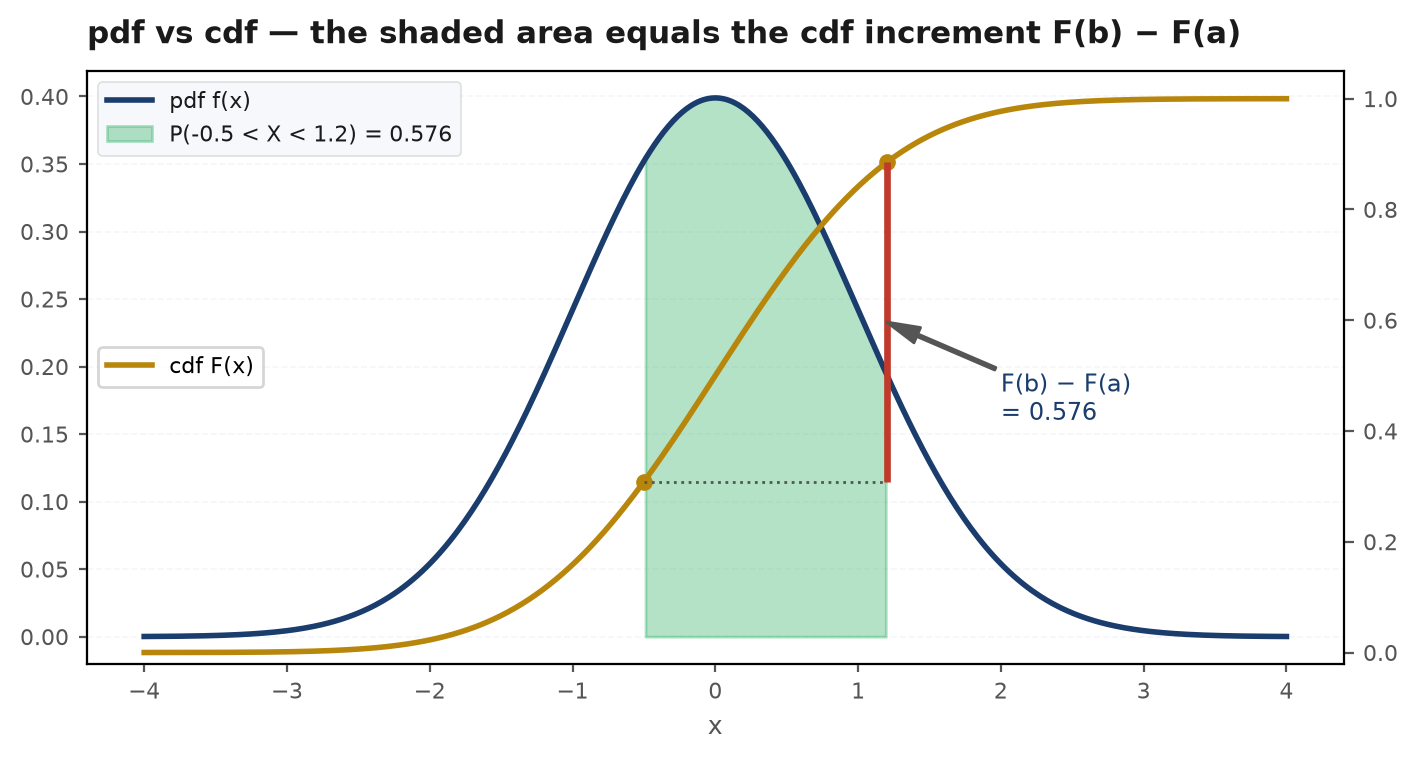
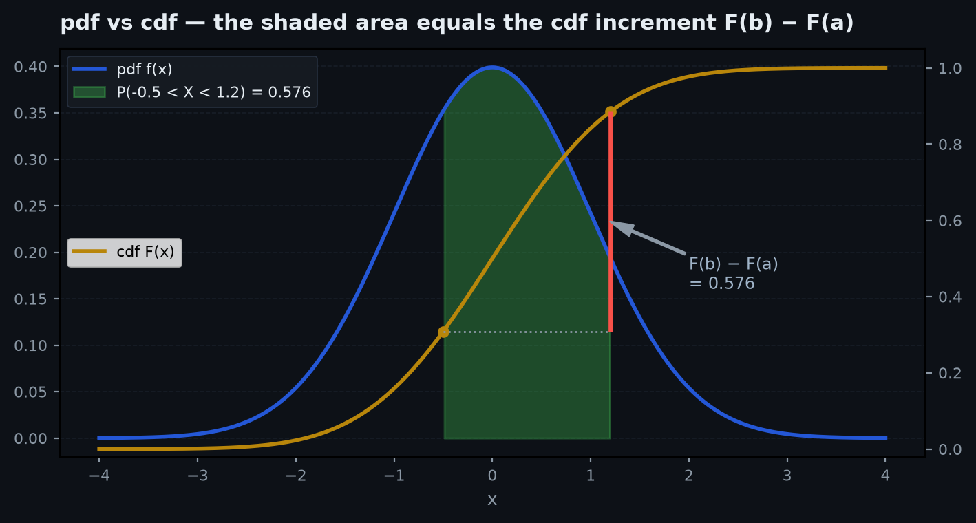
A probability density function above its cumulative distribution function, showing that area under the density equals the rise of the CDF and marking a quantile — The two faces of one distribution: area under the PDF over an interval (top) equals the rise of the CDF across it (bottom). The quantile function runs the CDF backwards — pick a probability on the vertical axis, read off the threshold. VaR is literally this arrow.

Running the CDF backwards gives the quantile function $Q (u) = F^{- 1} (u) = in f {x : F (x) \geq u}$ — the level that cuts off probability $u$ below. Quantiles are the language of risk: the 95% VaR of the applied probability chapter is $Q (0.95)$ of the loss distribution, and $F (X) \sim Uniform (0, 1)$ for continuous $F$ — the probability integral transform, proved in order statistics — grounds both simulation and p-values.

Transformations of random variables#

Given $Y = g (X)$ , what is $Y$ ’s distribution? The robust method works through the CDF; for monotone $g$ it yields a clean formula.

✦Proof — the change-of-variables formula

Let $g$ be strictly increasing and differentiable, with inverse $g^{- 1}$ . Then

F_{Y} (y) = P (g (X) \leq y) = P (X \leq g^{- 1} (y)) = F_{X} (g^{- 1} (y)) .

Differentiate with the chain rule:

f_{Y} (y) = f_{X} (g^{- 1} (y)) \frac{d}{d y} g^{- 1} (y) .

For decreasing $g$ the inequality flips, producing a minus sign that the absolute value absorbs. General monotone case:

f_{Y} (y) = f_{X} (g^{- 1} (y)) \frac{d g ^{- 1} ( y )}{d y} . ■

The Jacobian factor is conservation of probability: mass $f_{X} (x) d x$ in a small interval must reappear in the image interval of width $∣ g^{'} (x) ∣ d x$ — where $g$ stretches, density thins. Non-monotone maps (like $g (x) = x^{2}$ ) sum this over each monotone branch.

✦Worked example — from normal returns to lognormal prices

Let $X \sim N (μ, σ^{2})$ be a log return and $S = e^{X}$ the gross price relative. With $g^{- 1} (s) = ln s$ and derivative $1/ s$ :

f_{S} (s) = \frac{1}{s σ 2 π} exp (- \frac{( ln s - μ ) ^{2}}{2 σ ^{2}}), s > 0

— the lognormal density, the terminal distribution of geometric Brownian motion. The $1/ s$ Jacobian is what skews it right: equal log-moves map to wider dollar intervals on the upside. Its mean–median gap is derived in the zoo.

Expectation, linearity, and LOTUS#

The expectation is the probability-weighted average:

E [X] = x \sum x p (x) (discrete), E [X] = \int_{- \infty}^{\infty} x f (x) d x (continuous),

defined whenever the sum/integral converges absolutely — a caveat with teeth, as the St. Petersburg and Cauchy examples below show. Its superpower is linearity: $E [a X + bY] = a E [X] + b E [Y]$ , with no independence assumption whatsoever.

✦Proof — linearity needs no independence

Discrete case; let $p (x, y)$ be the joint PMF. By definition of the expectation of a function of $(X, Y)$ ,

E [a X + bY] = x \sum y \sum (a x + b y) p (x, y) = a x \sum x y \sum p (x, y) + b y \sum y x \sum p (x, y) .

The inner sums collapse to the marginals $p_{X} (x)$ and $p_{Y} (y)$ , leaving $a E [X] + b E [Y]$ . The joint distribution — where all dependence lives — was summed out without ever being factored. ■ This is why the indicator method later works on wildlydependent pieces, and why a book’s expected PnL is the sum of per-trade expectancies no matter how correlated the trades are (their risk is another story — joint distributions).

To average a function of $X$ you do not need the distribution of $g (X)$ — the law of the unconscious statistician (LOTUS) lets you integrate against $X$ ’s own distribution:

E [g (X)] = x \sum g (x) p (x) or \int g (x) f (x) d x .

It is a theorem, not a definition (its name is a joke about forgetting it needed proof), and note the trap it does not license: $E [g (X)] \neq = g (E [X])$ for nonlinear $g$ — the gap is Jensen’s inequality, quantified in inequalities & tail bounds, and it is the entire volatility-drag story ( $E [ln S] < ln E [S]$ ).

The tail-sum formula#

For a non-negative integer-valued variable there is a second, often far cleaner, route to the mean — summing the survival function:

E [X] = k = 1 \sum \infty P (X \geq k) .

✦Proof — swap the order of a double sum

Write $X = \sum_{k = 1}^{X} 1$ , i.e. $X = \sum_{k \geq 1} 1 {X \geq k}$ — the variable counts how many thresholds it clears. Take expectations and use linearity (fine for non-negative terms):

E [X] = k \geq 1 \sum E [1 {X \geq k}] = k \geq 1 \sum P (X \geq k) . ■

Equivalently: arrange the PMF as a table of $P (X = n)$ repeated $n$ times and sum by columns instead of rows. The continuous analogue, proved the same way with Fubini, is $E [X] = \int_{0}^{\infty} P (X > t) d t$ — the mean is the area under the survival curve.

✦Worked example — geometric mean in two lines

Let $X$ be the number of trials to the first success, success probability $p$ . Then $P (X \geq k) = (1 - p)^{k - 1}$ (the first $k - 1$ trials all fail), so

E [X] = k \geq 1 \sum (1 - p)^{k - 1} = \frac{1}{1 - ( 1 - p )} = \frac{1}{p} .

No differentiation of power series, no algebra. The tail-sum route is worth internalising — it also cracks “expected maximum of dice” (Problem 2 below) and any problem where $P (X \geq k)$ is easier than $P (X = k)$ .

Variance, covariance, and higher moments#

Variance measures spread as expected squared deviation, with the computational identity obtained by expanding the square and applying linearity:

Var (X) = E [(X - μ)^{2}] = E [X^{2}] - μ^{2}, μ = E [X] .

Its algebra, all one-line consequences of linearity:

$Var (a X + b) = a^{2} Var (X)$ — shifts do nothing, scales enter squared.
$Var (X + Y) = Var (X) + Var (Y) + 2 Cov (X, Y)$ , where $Cov (X, Y) = E [X Y] - E [X] E [Y]$ — variances add only when covariances vanish; that failure of linearity is diversification.

Standardised higher moments describe shape: skewness $E [(X - μ)^{3}] / σ^{3}$ (asymmetry — negative skew is the many-small-wins, rare-big-loss profile) and kurtosis $E [(X - μ)^{4}] / σ^{4}$ (tail weight — 3 for the normal, far above 3 for real returns). They are the moments where Sharpe ratios go blind, as the applied chapter shows on data.

✦Worked example — mean and variance of one die

$E [X] = \frac{1 + \dots + 6}{6} = \frac{21}{6} = 3.5$ ; $E [X^{2}] = \frac{1 + 4 + 9 + 16 + 25 + 36}{6} = \frac{91}{6}$ ; so $Var (X) = \frac{91}{6} - \frac{49}{4} = \frac{35}{12} \approx 2.917$ , $σ \approx 1.71$ . For the sum of two independent dice: mean 7, variance $35/6$ — add means always, add variances because independent. Memorise $35/12$ ; dice problems are standard practice furniture.

Moment generating functions#

The MGF packs every moment into one function:

M_{X} (t) = E [e^{tX}], finite for t in a neighbourhood of 0.

✦Proof sketch — moments from derivatives, and uniqueness

Expand the exponential and (where the expansion is justified) exchange expectation and sum:

M_{X} (t) = E [k \geq 0 \sum \frac{( tX ) ^{k}}{k !}] = k \geq 0 \sum \frac{E [ X ^{k} ]}{k !} t^{k} ⟹ M_{X}^{(k)} (0) = E [X^{k}] .

Differentiate $k$ times, set $t = 0$ , and the $k$ -th moment falls out. Uniqueness (stated, proof beyond scope): if the MGF is finite on an open interval around 0, it determines the distribution — two variables with the same MGF there are identically distributed. That, plus $M_{X + Y} = M_{X} M_{Y}$ for independent variables, is why MGFs demolish sum-of-variables problems and drive the CLT proof in LLN & CLT. ■

✦Derivation — the normal MGF by completing the square

For $Z \sim N (0, 1)$ :

M_{Z} (t) = \int \frac{e ^{t z}}{2 π} e^{- z^{2} /2} d z = e^{t^{2} /2} \int \frac{1}{2 π} e^{- (z - t)^{2} /2} d z = e^{t^{2} /2},

because $t z - z^{2} /2 = t^{2} /2 - (z - t)^{2} /2$ and the remaining integrand is a shifted normal density integrating to 1. Then for $X = μ + σ Z \sim N (μ, σ^{2})$ ,

M_{X} (t) = e^{μ t} M_{Z} (σ t) = exp (μ t + \frac{1}{2} σ^{2} t^{2}) . ■

Check the machinery: $M^{'} (0) = μ$ , $M^{''} (0) = μ^{2} + σ^{2}$ , so $Var = σ^{2}$ . Set $t = 1$ : $E [e^{X}] = e^{μ + σ^{2} /2}$ — the lognormal mean, volatility drag surfacing through an MGF. When the MGF fails to exist (Student-t, Cauchy, lognormal for $t > 0$ ), the characteristic function $φ_{X} (t) = E [e^{i tX}]$ — always finite, always unique — takes over; it is the tool of record in the CLT chapter.

The indicator-variable method#

The most useful trick in this entire series. An indicator $1_{A}$ is 1 when $A$ occurs, else 0, and its expectation is a probability: $E [1_{A}] = P (A)$ . To find an expected count, write it as a sum of indicators and apply linearity — dependence between the events is irrelevant:

X = i = 1 \sum n 1_{A_{i}} ⟹ E [X] = i = 1 \sum n P (A_{i}) .

Matches (fixed points). A random permutation of $n$ items: $P (item i fixed) = 1/ n$ , so the expected number of fixed points is $n \cdot \frac{1}{n} = 1$ — for every $n$ , despite the heavy dependence (compare the derangement count in counting & combinatorics).
Empty boxes. Throw $n$ balls into $n$ boxes uniformly: $P (box j empty) = (1 - \frac{1}{n})^{n}$ , so the expected number of empty boxes is $n (1 - \frac{1}{n})^{n} \to n / e \approx 0.368 n$ — the bootstrap’s “36.8% of observations left out of a resample.”
Inversions. In a random permutation, each of the $(2 n)$ pairs is inverted with probability $1/2$ (symmetry), so the expected inversion count is $\frac{1}{2} (2 n) = \frac{n ( n - 1 )}{4}$ .

→Quant lens — expectancy decomposes; risk does not

Linearity over indicators is how a desk reasons about aggregates without modelling dependence: the expected number of stopped-out positions today is the sum of per-position stop probabilities; a book’s expectancy is the sum of per-trade edges (the math of edge) even when every trade loads on the same regime. But remember the boundary: the moment the question involves variance, drawdown, or tails, the vanished covariances return with interest — 100 correlated 1R bets have the expectancy of 100 trades and the risk of far fewer independent ones. Expected values need no correlation model; risk numbers are nothing but one.

A seeded simulation confirms three headline results — fixed points, the geometric tail-sum mean, and the empty-box $1/ e$ fraction:

moments_checks.py

import numpy as np

rng = np.random.default_rng(11)
trials = 200_000

# 1) Expected fixed points of a random permutation of n = 52 items: exactly 1
n = 52
perms = np.argsort(rng.random((trials, n)), axis=1)
fixed = (perms == np.arange(n)).sum(axis=1)
print(f"E[fixed points] = {fixed.mean():.4f}   (theory 1)")

# 2) Geometric mean via simulation: trials to first six, p = 1/6
rolls = rng.geometric(1/6, size=trials)
print(f"E[rolls to a 6] = {rolls.mean():.4f}   (theory 6)")
# tail-sum check: sum_k P(X >= k) computed empirically
ks = np.arange(1, 61)
tail_sum = np.array([(rolls >= k).mean() for k in ks]).sum()
print(f"sum P(X >= k)   = {tail_sum:.4f}   (same number, by the tail-sum formula)")

# 3) Empty boxes: n balls in n boxes, expected empty fraction -> 1/e
m = 100
boxes = rng.integers(0, m, size=(trials // 10, m))
empty_frac = np.array([m - len(np.unique(row)) for row in boxes]).mean() / m
print(f"empty fraction  = {empty_frac:.4f}   ((1-1/m)^m = {(1 - 1/m)**m:.4f}, 1/e = {1/np.e:.4f})")

Practice problems#

Five classics of expectation — each has a grind-it-out route and a slick route; lead with the slick one.

→Problem 1 — Expected rolls to see a 6

Roll a fair die repeatedly. How many rolls, on average, until the first 6?

Solution. Slick (first-step / memorylessness): let $E$ be the answer. The first roll either succeeds (probability $1/6$ ) or fails and — because the die has no memory — leaves you facing the identical problem, one roll poorer: $E = 1 + \frac{5}{6} E \Rightarrow E = 6$ . Systematic: geometric with $p = 1/6$ , tail-sum gives $\sum_{k} (5/6)^{k - 1} = 6$ . Be ready for the follow-up: after 10 non-sixes the expected number of additional rolls is still 6 (Problem 5) — contrast the all-even conditional of the axioms chapter, where conditioning on the future changed everything.

→Problem 2 — Expected maximum of two dice

Roll two fair dice. What is the expected value of the larger one?

Solution. Tail-sum on $M = max$ : $P (M \geq k) = 1 - P (both < k) = 1 - (\frac{k - 1}{6})^{2}$ . So

E [M] = k = 1 \sum 6 (1 - (\frac{k - 1}{6})^{2}) = 6 - \frac{0 + 1 + 4 + 9 + 16 + 25}{36} = 6 - \frac{55}{36} = \frac{161}{36} \approx 4.47.

Sanity checks worth running: above 3.5, below 6, and by the symmetry $min + max = X_{1} + X_{2}$ , $E [min] = 7 - \frac{161}{36} = \frac{91}{36} \approx 2.53$ — two answers for one. The CDF-of-the-max move generalises to any number of dice and to order statistics at large.

→Problem 3 — Coupon collector, via indicators

Each cereal box contains one of $n$ coupon types, uniformly at random. How many boxes on average to collect all $n$ ? Evaluate for $n = 6$ (rolling a die until every face appears).

Solution. Decompose into stages: with $k$ types already collected, each box is new with probability $\frac{n - k}{n}$ , so the stage is geometric with mean $\frac{n}{n - k}$ . Linearity across stages:

E [T] = k = 0 \sum n - 1 \frac{n}{n - k} = n j = 1 \sum n \frac{1}{j} = n H_{n} \approx n (ln n + 0.5772) .

For $n = 6$ : $6 (1 + \frac{1}{2} + \frac{1}{3} + \frac{1}{4} + \frac{1}{5} + \frac{1}{6}) = 6 \cdot \frac{49}{20} = 14.7$ rolls. The last coupon alone costs $n$ boxes on average — completeness is expensive. Full treatment in the brainteaser canon.

→Problem 4 — St. Petersburg: infinite mean, finite price

A fair coin is flipped until the first head; if it lands on flip $n$ you are paid $2^{n}$ . What is the fair price of this game?

Solution. $E = \sum_{n \geq 1} 2^{- n} \cdot 2^{n} = \sum_{n \geq 1} 1 = \infty$ — yet nobody pays more than about $20. The resolutions to present: (i) expectation means an absolutely convergent sum, and this one diverges — the “mean” is not a usable summary; (ii) any real counterparty is finitely capitalised — capping the bank at $2^{30}$ (~$1B) truncates the sum to 30, a ~$30 game; (iii) log utility (Bernoulli’s fix) gives a modest certainty equivalent — the concavity that drives Kelly sizing in position sizing. The quant moral: a payoff dominated by vanishingly rare astronomical outcomes has an expectation no realisable sample mean approaches — a first sighting of the fat-tail failures in LLN & CLT.

→Problem 5 — Memorylessness, precisely

For geometric $X$ (trials to first success), show $P (X > m + k ∣ X > m) = P (X > k)$ , and use it to re-derive $E [X] = 1/ p$ .

Solution. Since $P (X > k) = (1 - p)^{k}$ ,

P (X > m + k ∣ X > m) = \frac{( 1 - p ) ^{m + k}}{( 1 - p ) ^{m}} = (1 - p)^{k} = P (X > k) .

Past failures carry zero information — the process restarts at every trial. For the mean, condition on the first trial: $E [X] = p \cdot 1 + (1 - p) (1 + E [X])$ , since after a failure the memoryless clock restarts. Solving gives $E [X] = 1/ p$ . The geometric is the only discrete distribution with this property (the exponential is its continuous twin — uniqueness proved in the distribution zoo), and it is the clean rebuttal of the gambler’s fallacy: “due” is precisely what memorylessness forbids.

Next: the indicator method you just met deserves a chapter of its own — linearity of expectation as a first-class problem-solving tool, with the classic problems it demolishes. Expectation & the linearity trick.