Order statistics & extremes

Sort a sample and every position in the sorted list becomes a random variable with its own distribution: the minimum, the maximum, the median, the second-highest bid in an auction, the best-looking strategy out of fifty. Order statistics are the calculus of ranked randomness — and because trading constantly selects extremes (best backtest, worst drawdown, record high), their distributions are the honest answer to “how good should the best one look by luck alone?” This chapter derives the k-th order statistic’s distribution, the Beta law for uniforms, the probability integral transform, the $2 ln n$ growth of Gaussian maxima, records, and the German tank problem.

✦Intuition — the maximum is a biased estimator of quality

Ask fifty coin-flippers to flip twenty times each and the best of them will get around fifteen heads — not because anyone is skilled, but because you selected the maximum. The maximum of $n$ draws is pushed into the tail by construction, and its distribution tells you exactly how far. Everything in this chapter is a version of that one calculation, and the punchline for quants is uncomfortable: the expected best of $n$ zero-edge strategies grows like $2 ln n$ — slowly, but never zero. Selection is a source of apparent performance.

The distribution of the k-th order statistic#

Let $X_{1}, \dots, X_{n}$ be i.i.d. with CDF $F$ and density $f$ , and let $X_{(1)} \leq X_{(2)} \leq \dots \leq X_{(n)}$ be the sorted values. The key observation is a counting one: the event ${X_{(k)} \leq x}$ happens exactly when at least $k$ of the $n$ draws land at or below $x$ . The number that do is Binomial( $n, F (x)$ ), so

F_{X_{(k)}} (x) = P (X_{(k)} \leq x) = j = k \sum n (j n) F (x)^{j} (1 - F (x))^{n - j} .

The two ends are the cases to know cold — they need no summation:

F_{X_{(n)}} (x) = F (x)^{n} (all n below x), F_{X_{(1)}} (x) = 1 - (1 - F (x))^{n} (not all above) .

✦Proof sketch — the density of the k-th order statistic

Differentiating the sum works but is messy. The direct argument: for $X_{(k)}$ to land in the sliver $[x, x + d x]$ , one draw must fall in the sliver (probability $f (x) d x$ ), exactly $k - 1$ must fall below (probability $F (x)^{k - 1}$ ), and the remaining $n - k$ above (probability $(1 - F (x))^{n - k}$ ). The number of ways to assign draws to the three roles is the multinomial coefficient $(k - 1 , 1 , n - k n) = \frac{n !}{( k - 1 )! 1 ! ( n - k )!}$ . Multiply:

f_{X_{(k)}} (x) = \frac{n !}{( k - 1 )! ( n - k )!} F (x)^{k - 1} (1 - F (x))^{n - k} f (x) . ■

(Two draws in the sliver has probability of order $(d x)^{2}$ — negligible. This “one here, count the rest” pattern is the same combinatorial move as stars and bars, and it is worth being able to reproduce it from scratch in one line.)

Worked example (by hand). Three independent $U (0, 1)$ draws. Probability the maximum is below 0.9: $0. 9^{3} = 0.729$ . Probability the minimum exceeds 0.5: $0. 5^{3} = 0.125$ . Density of the maximum: $f_{(3)} (x) = 3 x^{2}$ , so $E [X_{(3)}] = \int_{0}^{1} 3 x^{3} d x = 3/4$ . The maximum of three uniforms sits, on average, three-quarters of the way up — each extra draw pushes the record closer to 1, but with diminishing returns.

Uniform order statistics — the Beta law and spacings#

For uniforms, $F (x) = x$ on $[0, 1]$ and the general density specialises to something famous. Substituting into the boxed density:

f_{X_{(k)}} (x) = \frac{n !}{( k - 1 )! ( n - k )!} x^{k - 1} (1 - x)^{n - k} ⟹ X_{(k)} \sim Beta (k, n + 1 - k) .

This is the Beta distribution’s origin story (see the distribution zoo): Beta( $a, b$ ) is the law of the $a$ -th smallest of $a + b - 1$ uniforms. From the Beta mean $a / (a + b)$ :

E [X_{(k)}] = \frac{k}{n + 1}, E [X_{(1)}] = \frac{1}{n + 1}, E [X_{(n)}] = \frac{n}{n + 1} .

✦The slick symmetry argument for k/(n+1)

No integration needed: $n$ uniform points cut $[0, 1]$ into $n + 1$ spacings. By symmetry (exchangeability of the gaps — rotate the circle obtained by gluing 0 to 1), all $n + 1$ spacings have the same distribution, and they sum to 1, so each has expectation $1/ (n + 1)$ . Then $X_{(k)}$ is the sum of the first $k$ spacings: $E [X_{(k)}] = k / (n + 1)$ . The sorted uniforms sit, on average, at perfectly even quantile positions — this is why p-p plots and $k / (n + 1)$ plotting positions work. Each single spacing is $Beta (1, n)$ , i.e. $P (gap > x) = (1 - x)^{n}$ — for large $n$ , approximately exponential with rate $n$ , the bridge to Poisson-process interarrivals.

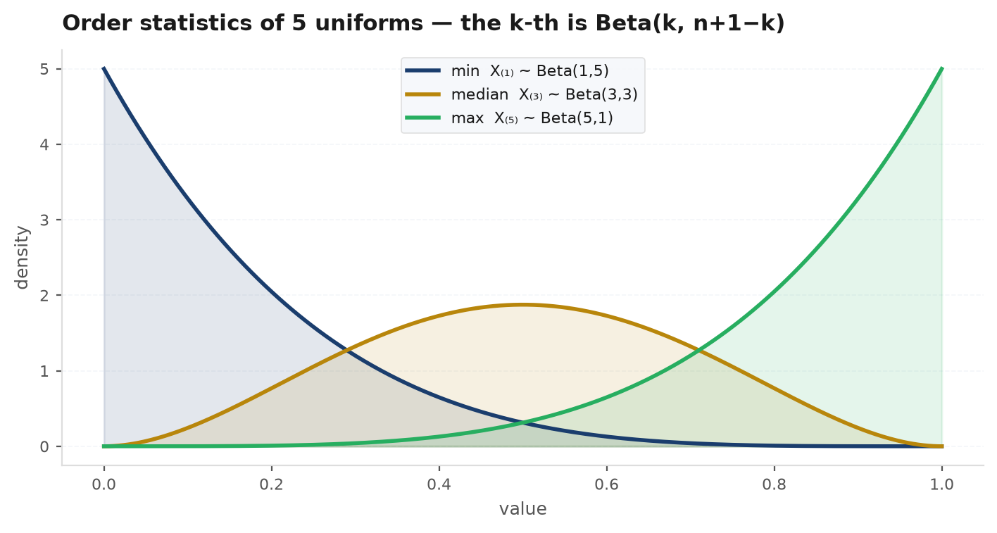
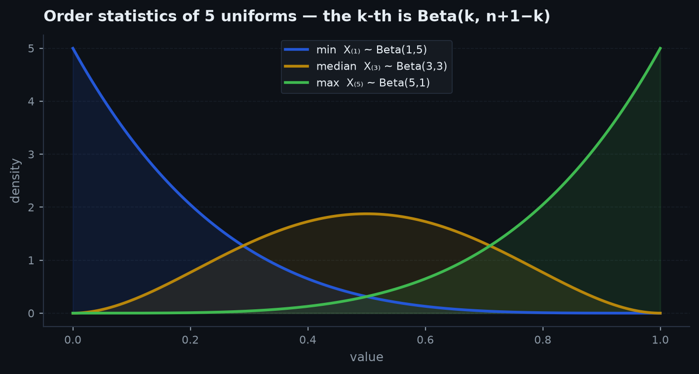
Beta densities of the order statistics of uniform samples, showing the minimum, median, and maximum densities peaking at evenly spaced positions — Densities of the order statistics of n uniforms: X_(k) ~ Beta(k, n+1-k). The minimum and maximum hug the edges, the median peaks in the centre, and the means line up at the even quantile positions k/(n+1). Sorting turns one flat distribution into a fan of sharply located ones.

The range $R = X_{(n)} - X_{(1)}$ follows immediately: $E [R] = \frac{n}{n + 1} - \frac{1}{n + 1} = \frac{n - 1}{n + 1}$ . Ten uniform draws span, on average, $9/11 \approx 82%$ of the interval.

The probability integral transform#

One theorem explains why uniforms are the universal currency of simulation and of p-values.

✦Proof — F(X) is uniform, and F⁻¹(U) has law F

Let $X$ have a continuous, strictly increasing CDF $F$ , and set $U = F (X)$ . For any $u \in (0, 1)$ ,

P (U \leq u) = P (F (X) \leq u) = P (X \leq F^{- 1} (u)) = F (F^{- 1} (u)) = u,

which is exactly the $U (0, 1)$ CDF. Conversely, if $U \sim U (0, 1)$ then $P (F^{- 1} (U) \leq x) = P (U \leq F (x)) = F (x)$ , so $F^{- 1} (U)$ has CDF $F$ . $■$ (For general $F$ , use the generalised inverse $F^{- 1} (u) = in f {x : F (x) \geq u}$ ; the second statement survives untouched.)

Two consequences. Simulation: to sample any distribution, sample a uniform and push it through $F^{- 1}$ — the inverse-transform method of Monte Carlo. Inference: a p-value is $1 - F_{0} (T)$ for a test statistic $T$ with null CDF $F_{0}$ , so under the null the p-value is exactly Uniform(0,1) — the fact that makes p-value thresholds meaningful and multiple-testing corrections computable (multiple testing & paradoxes).

How big is the maximum? Gaussian extremes#

For uniforms the maximum crawls toward the endpoint. For unbounded distributions the question is how fast the maximum grows, and for Gaussians there is a clean, classic answer.

✦Heuristic derivation — E[max] of n standard normals ≈ √(2 ln n)

The maximum of $n$ draws sits near the level $t$ that a single draw exceeds about once in $n$ tries — i.e. solve $n P (X > t) \approx 1$ . Using the Gaussian tail approximation $P (X > t) \approx \frac{φ ( t )}{t} = \frac{1}{t 2 π} e^{- t^{2} /2}$ , take logs of $n e^{- t^{2} /2} \approx t 2 π$ :

ln n - \frac{t ^{2}}{2} \approx ln (t 2 π) ⟹ t^{2} \approx 2 ln n - O (ln ln n) ⟹ E [max] \sim 2 ln n .

The correction terms are negative and decay slowly, so $2 ln n$ overstates the mean at practical $n$ (see the table) — but the growth rate is right, and the qualitative fact is the one to internalise: the max of Gaussians grows only logarithmically. Doubling your number of tries barely moves the record; and fluctuations of the max stay $O (1/ 2 ln n)$ — the max concentrates. The full limit theory (Gumbel, Fréchet, Weibull) is in extreme value theory.

n	√(2 ln n)	E[max] (exact/simulated)
10	2.15	1.54
100	3.03	2.51
1,000	3.72	3.24
1,000,000	5.26	4.86

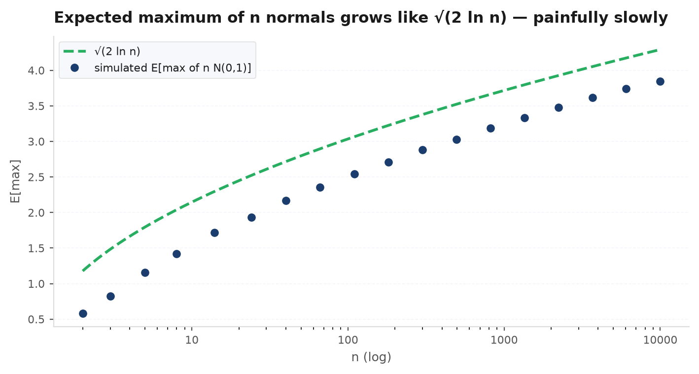
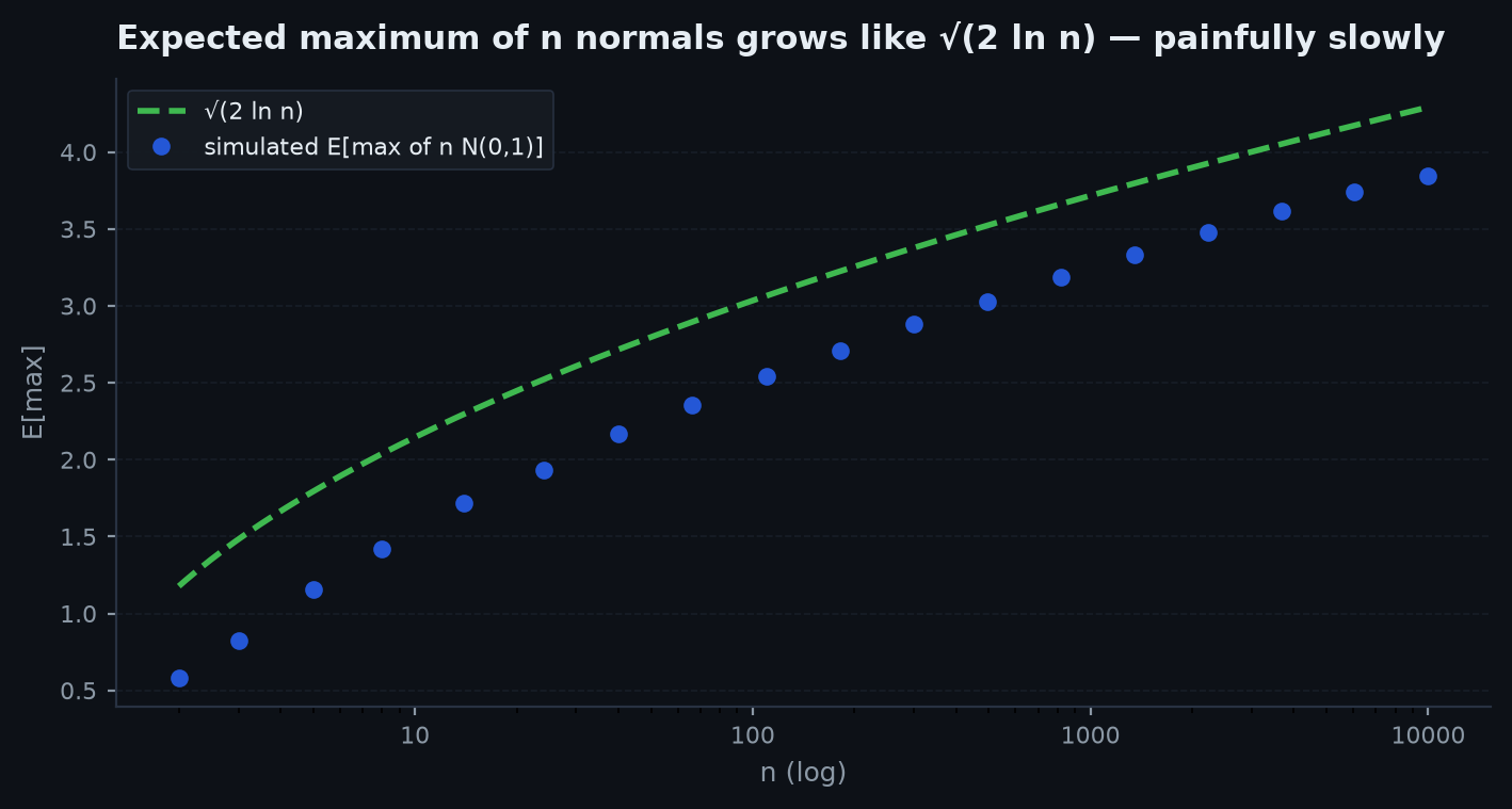
Expected maximum of n standard normal draws plotted against n on a log scale, growing like the square root of two log n, with the asymptote drawn above the exact curve — The expected maximum of n standard normals grows like sqrt(2 ln n) — painfully slowly, with the asymptote (upper curve) approached from below. Selection inflates the best observation, but only logarithmically: the 1000th strategy you try moves the luck ceiling far less than the 10th did.

→Quant lens — the best backtest of N is a max, not a mean

Test $N$ independent zero-edge strategies and each produces a roughly Gaussian Sharpe t-stat. The best one is the max of $N$ Gaussians: expected value $\approx 2 ln N$ standard errors — about 2.1 for $N = 10$ , 3.0 for $N = 100$ . So “our best strategy has t = 3” is the expected outcome of trying a hundred random ones. This is the mathematical core of data snooping, the deflated Sharpe ratio, and the reason overfitting detectionasks “how many did you try?” before it asks anything else. Same math, different market: the winning bid in an auction and the highest-water-mark fund in a database are maxima too — both flattered by exactly this amount.

Records — 1/n by pure symmetry#

Observation $n$ sets a record if it exceeds all before it: $X_{n} > max (X_{1}, \dots, X_{n - 1})$ .

✦Proof — P(record at n) = 1/n, and E[# records] = H_n

Among the exchangeable draws $X_{1}, \dots, X_{n}$ (i.i.d., continuous so no ties), each is equally likely to be the largest, so $P (X_{n} is the largest of the first n) = 1/ n$ — no calculation, pure symmetry. With indicator variables $I_{n} = 1 {record at n}$ and linearity of expectation (the workhorse of random variables & moments):

E [# records in n draws] = m = 1 \sum n \frac{1}{m} = H_{n} \approx ln n + 0.5772. ■

A century of annual data yields $H_{100} \approx 5.19$ expected records — record heat, record volume, record drawdown are frequent under pure randomness, and (a lovely deeper fact) the record indicators are mutually independent. When a desk celebrates a “record month,” the base-rate question is $1/ n$ , not zero.

The German tank problem#

Order statistics power one of the great applied-statistics war stories. Serial numbers $1, \dots, N$ with $N$ unknown; you capture $k$ tanks — a sample without replacement — and observe maximum serial $m$ . The maximum alone is the sufficient statistic, but $m$ itself is biased low (the max of a sample never exceeds, and rarely equals, the max of the population). The expected gap above $m$ should equal the average spacing: the $k$ observed serials cut $1.. N$ into $k + 1$ nearly-equal gaps, so $E [m] = \frac{k}{k + 1} (N + 1) - \frac{1}{2}$ roughly — solving gives the unbiased (indeed UMVU) estimator

N^= m (1 + \frac{1}{k}) - 1 = m + \frac{m - k}{k} .

Worked example. Five captured tanks, highest serial 60: $N^= 60 \cdot 1.2 - 1 = 71$ . Read the second form: take the observed max and add the average observed gap ( $(60 - 5) /5 = 11$ ) — the sample’s own spacing estimates how far beyond the sample the population extends. In WWII this estimator put German tank production near 270/month while intelligence guessed 1,400; records later showed 276. The same logic prices “how many competitors are in this trade” from the sparse ones you can see.

order_stats_check.py

import numpy as np

rng = np.random.default_rng(11)
reps = 100_000

# 1) k-th order statistic of uniforms is Beta(k, n+1-k): check k=2, n=5
u = np.sort(rng.random(size=(reps, 5)), axis=1)
x2 = u[:, 1]                                   # X_(2) of n=5 -> Beta(2, 4)
print(f"X_(2) of 5 uniforms: mean={x2.mean():.4f} (theory 2/6={2/6:.4f}), "
      f"var={x2.var():.5f} (theory {2*4/(6**2*7):.5f})")

# 2) E[max of n normals] vs the sqrt(2 ln n) asymptote
for n in (10, 100, 1000):
    mx = rng.standard_normal(size=(20_000, n)).max(axis=1)
    print(f"n={n:5d}  E[max]={mx.mean():.3f}   sqrt(2 ln n)={np.sqrt(2*np.log(n)):.3f}")

# 3) Records: expected count in n draws = H_n = 1 + 1/2 + ... + 1/n
n = 100
x = rng.standard_normal(size=(reps, n))
records = (x >= np.maximum.accumulate(x, axis=1)).sum(axis=1)
print(f"records in {n} draws: {records.mean():.3f}  (H_100 = {sum(1/i for i in range(1, n+1)):.3f})")

Practice problems#

→Problem 1 — expected max of two (and three) uniforms

$X, Y \sim U (0, 1)$ independent. Find $E [max (X, Y)]$ ; then for three uniforms.

Solution. Systematic: $F_{m a x} (x) = x^{2}$ , density $2 x$ , so $E [max] = \int_{0}^{1} 2 x^{2} d x = 2/3$ ; for three, $\int_{0}^{1} 3 x^{3} d x = 3/4$ . Slick: by the spacings symmetry, $E [X_{(k)}] = k / (n + 1)$ , giving $2/3$ and $3/4$ instantly — and the general answer $n / (n + 1)$ for the max of $n$ . Worth adding unprompted: $E [min] = 1/ (n + 1)$ , and $E [max] + E [min] = 1$ by the symmetry $x \mapsto 1 - x$ — a one-line sanity check worth making a habit.

→Problem 2 — expected number of records

You observe 100 i.i.d. yearly returns. How many record years (each beating all previous) do you expect? Why does the answer not depend on the return distribution?

Solution. Record at year $m$ has probability $1/ m$ — among $m$ exchangeable continuous draws, each is equally likely to be largest, so the distribution cancels out entirely. By linearity of expectation over the indicators (dependence irrelevant): $E = H_{100} = 1 + \frac{1}{2} + \dots + \frac{1}{100} \approx 5.19$ . About five record years per century — logarithmic growth, so records keep arriving forever, just ever more rarely. Follow-up they like: the probability year 100 itself is a record is exactly $1/100$ , distribution-free — the cleanest nonparametric test statistic there is.

→Problem 3 — broken stick, triangle

Break a unit stick at two points chosen uniformly at random. What is the probability the three pieces form a triangle?

Solution. Let the cut points be $U_{(1)} < U_{(2)}$ (the order statistics of two uniforms); pieces are $U_{(1)}, U_{(2)} - U_{(1)}, 1 - U_{(2)}$ . A triangle exists iff every piece is shorter than $\frac{1}{2}$ (each side must be beaten by the other two summing past it). In the $(u_{1}, u_{2})$ unit square the failure regions — some piece $\geq \frac{1}{2}$ — carve out three corner triangles of total area $\frac{3}{4}$ , leaving

P (triangle) = \frac{1}{4} .

Fast symmetry version: the three “a piece exceeds ½” events are disjoint and each has probability $\frac{1}{4}$ (both cuts must land in the same half-stick region), so the failure probability is $\frac{3}{4}$ . Classic enough that the escalation — “break the longer piece again instead” — should be expected; the machinery is identical, only the conditioning changes.

→Problem 4 — the second-highest bid

$n$ bidders draw private values i.i.d. $U (0, 1)$ . In a second-price auction (winner pays the second-highest value), what revenue does the seller expect?

Solution. Truthful bidding is dominant in a second-price auction, so revenue is the second order statistic from the top: $X_{(n - 1)} \sim Beta (n - 1, 2)$ , hence

E [revenue] = E [X_{(n - 1)}] = \frac{n - 1}{n + 1} .

Two bidders: $1/3$ ; five: $2/3$ ; the gap to the highest value $n / (n + 1)$ — the winner’s information rent — is exactly one average spacing, $1/ (n + 1)$ , shrinking as competition thickens. The market intuition transfers directly to order books: the spread you pay crossing to the best quote behaves like a top spacing, and it tightens as the number of competing quotes grows.

→Problem 5 — the median of three uniforms

Three i.i.d. $U (0, 1)$ draws. Find the distribution, mean, and variance of the median.

Solution. $X_{(2)}$ with $n = 3, k = 2$ is $Beta (2, 2)$ : density $f (x) = \frac{3 !}{1 ! 1 !} x (1 - x) = 6 x (1 - x)$ — an inverted parabola peaking at $\frac{1}{2}$ . Mean $\frac{1}{2}$ by symmetry (or $k / (n + 1) = 2/4$ ); variance from the Beta formula $\frac{ab}{( a + b ) ^{2} ( a + b + 1 )} = \frac{4}{16 \cdot 5} = \frac{1}{20}$ . Compare a single draw: variance $1/12$ . The median of three is a better estimator of the centre than one draw (variance down 40%) yet uses no arithmetic on the values — the germ of robust statistics, and of why median-based statistics resist outliers that wreck means.

Next: from sorted randomness to sequential randomness — fair games, stopping rules, and the theorem that says no exit strategy can beat a game with no edge: Martingales & optional stopping.