The distribution zoo

Every named distribution is a story about how randomness gets generated — coin flips accumulated, waiting times elapsed, rare events counted, errors averaged. Good problems test the stories, not just the formulas. This chapter walks the whole zoo — sixteen distributions — deriving the non-obvious moments, proving the two memorylessness results, and tying each animal to where it appears on a trading desk.

✦Intuition — a distribution is a mechanism, not a formula

Nobody memorises sixteen pmfs cold. What you memorise is sixteen mechanisms: a Binomial is “count successes in independent tries”, a Geometric is “wait for the first success”, a Poisson is “count rare events at a constant rate”. Name the mechanism and the formulas, moments, and limit theorems reconstruct themselves — story first, algebra second.

A grid of small plots showing the pmf or pdf of the major named distributions: Bernoulli, Binomial, Geometric, Poisson, Uniform, Exponential, Gamma, Beta, Normal, Lognormal, Student-t, and Pareto — The zoo at a glance. Discrete pmfs on top, continuous pdfs below. Every one of these is the answer to a ‘which distribution models X?’ question for some mechanism X.

Discrete distributions#

Bernoulli and Binomial#

A Bernoulli $(p)$ variable is a single yes/no experiment: $P (X = 1) = p$ , $P (X = 0) = 1 - p$ . Its moments are immediate — $E [X] = p$ and, since $X^{2} = X$ , $Var (X) = p (1 - p)$ . A Binomial $(n, p)$ counts successes in $n$ independent trials:

P (X = k) = (k n) p^{k} (1 - p)^{n - k}, k = 0, 1, \dots, n .

Writing $X = \sum_{i = 1}^{n} X_{i}$ as a sum of indicators — the workhorse trick from Random variables & moments — linearity gives $E [X] = n p$ with no combinatorics, independence gives $Var (X) = n p (1 - p)$ , and the MGF factorises to $M_{X} (t) = (1 - p + p e^{t})^{n}$ . In finance the Binomial is the win/loss record of $n$ trades and the lattice of the binomial option-pricing tree.

Geometric#

The Geometric $(p)$ waits for the first success: $P (X = k) = (1 - p)^{k - 1} p$ . Its tail is clean — $P (X > k) = (1 - p)^{k}$ , the probability of $k$ straight failures — and the tail-sum formula gives the mean instantly:

E [X] = k = 0 \sum \infty P (X > k) = k = 0 \sum \infty (1 - p)^{k} = \frac{1}{p}, Var (X) = \frac{1 - p}{p ^{2}} .

✦Proof — the Geometric is memoryless

Claim: $P (X > m + n ∣ X > m) = P (X > n)$ . Proof: using $P (X > k) = (1 - p)^{k}$ ,

P (X > m + n ∣ X > m) = \frac{P ( X > m + n )}{P ( X > m )} = \frac{( 1 - p ) ^{m + n}}{( 1 - p ) ^{m}} = (1 - p)^{n} = P (X > n) . ■

Past failures tell you nothing about the remaining wait — the process restarts fresh at every step. It is the only discrete distribution on ${1, 2, \dots}$ with this property (the tail must satisfy $g (m + n) = g (m) g (n)$ , forcing $g (k) = q^{k}$ ) — the rigorous gambler’s-fallacy rebuttal from Axioms, conditioning & Bayes: a fair game owes you nothing.

Negative binomial#

Wait for the $r$ -th success and you get the Negative binomial $(r, p)$ : the last trial is a success, the preceding $k - 1$ hold exactly $r - 1$ successes,

P (X = k) = (r - 1 k - 1) p^{r} (1 - p)^{k - r}, k = r, r + 1, \dots

Since $X$ is a sum of $r$ independent Geometrics (wait, restart, repeat), linearity gives $E [X] = r / p$ and $Var (X) = r (1 - p) / p^{2}$ — no new derivation needed. With variance exceeding its mean, it is the standard model for overdispersed counts (trade arrivals that cluster more than Poisson allows).

Hypergeometric#

Sample $n$ items without replacement from $N$ containing $K$ successes; the successes drawn are Hypergeometric:

P (X = k) = \frac{( k K ) ( n - k N - K )}{( n N )}, E [X] = n \frac{K}{N}, Var (X) = n \frac{K}{N} (1 - \frac{K}{N}) \frac{N - n}{N - 1} .

The mean follows from indicators — each draw is marginally a success with probability $K / N$ by symmetry, despite the dependence. The variance carries the finite-population correction $(N - n) / (N - 1)$ : sampling without replacement shrinks variance, and as $N \to \infty$ it converges to the Binomial. It prices card counting and any “pick from a finite universe” setup — selecting stocks from an index containing $K$ eventual winners.

Poisson#

The Poisson $(λ)$ counts rare events at a constant rate:

P (X = k) = e^{- λ} \frac{λ ^{k}}{k !}, E [X] = Var (X) = λ, M_{X} (t) = e^{λ (e^{t} - 1)} .

✦Proof sketch — Poisson as the limit of Binomials (law of rare events)

Let $X_{n} \sim Binomial (n, λ / n)$ : many trials, tiny success probability, mean fixed at $λ$ . For fixed $k$ ,

P (X_{n} = k) = (k n) (\frac{λ}{n})^{k} (1 - \frac{λ}{n})^{n - k} = \to 1 \frac{n ( n - 1 ) \dots ( n - k + 1 )}{n ^{k}} \cdot \frac{λ ^{k}}{k !} \cdot \to e^{- λ} (1 - \frac{λ}{n})^{n} \cdot \to 1 (1 - \frac{λ}{n})^{- k} ⟶ e^{- λ} \frac{λ ^{k}}{k !} . ■

The Poisson therefore approximates any “many chances, each unlikely” count — bond defaults, limit-order arrivals, birthday collisions — with error $O (λ^{2} / n)$ , excellent whenever $p ≲ 0.05$ .

Worked example.200 bonds each default independently with probability 1.5% per year. The count is Binomial(200, 0.015) ≈ Poisson( $λ = 3$ ); at most one default:

P (X \leq 1) \approx e^{- 3} (1 + 3) = 4 e^{- 3} \approx 0.199,

versus the exact Binomial answer 0.1963. Poisson counts also add: independent rates sum to a Poisson with rate $λ_{1} + λ_{2}$ (multiply the MGFs) — the superposition property of Poisson processes.

Continuous distributions#

Uniform#

The Uniform $(a, b)$ has constant density $1/ (b - a)$ , with $E [X] = (a + b) /2$ and $Var (X) = (b - a)^{2} /12$ (the 12 is worth memorising). Its real importance is as the source of all randomness: for any CDF $F$ , $F^{- 1} (U)$ has distribution $F$ — the inverse-transform method behind every Monte-Carlo engine and the probability integral transform behind p-values (Order statistics & extremes).

Exponential#

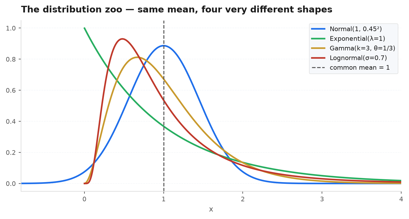
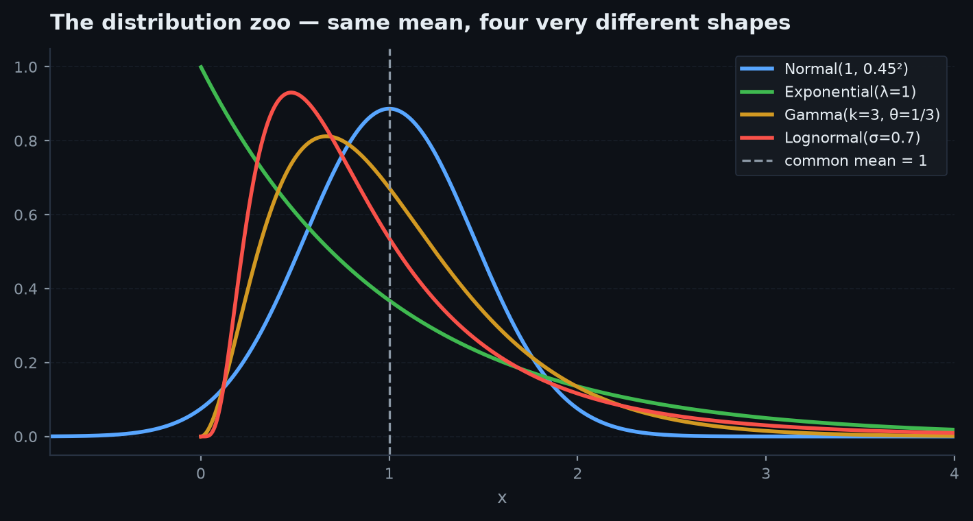
The Exponential $(λ)$ is the continuous waiting time — the Geometric’s limit as steps shrink:

f (x) = λ e^{- λ x}, x \geq 0; P (X > x) = e^{- λ x}; E [X] = \frac{1}{λ}, Var (X) = \frac{1}{λ ^{2}} .

✦Proof — memorylessness, and why the Exponential is the only one

Memoryless: $P (X > s + t ∣ X > s) = e^{- λ (s + t)} / e^{- λ s} = e^{- λ t} = P (X > t) .$ Uniqueness: write $g (t) = P (X > t)$ ; memorylessness says $g (s + t) = g (s) g (t)$ . Then $g (m / n) = g (1/ n)^{m} = g (1)^{m / n}$ for all rationals by induction, and right-continuity of survival functions extends this to all reals: $g (t) = g (1)^{t} = e^{- λ t}$ with $λ = - ln g (1) > 0$ . The functional equation has no other monotone solution — memorylessness is the exponential. $■$

Two facts do heavy duty in problems. Minimum: for independent $X_{i} \sim Exp (λ_{i})$ , $P (min_{i} X_{i} > t) = \prod_{i} e^{- λ_{i} t} = e^{- (\sum_{i} λ_{i}) t}$ — the minimum is Exponential with the summed rate. Race: $P (X_{1} < X_{2}) = λ_{1} / (λ_{1} + λ_{2})$ . Both are solved below.

Gamma#

Sum $k$ independent Exponential $(λ)$ waits and you get the Gamma $(k, λ)$ (the Erlang when $k$ is an integer):

f (x) = \frac{λ ^{k} x ^{k - 1} e ^{- λ x}}{Γ ( k )}, E [X] = \frac{k}{λ}, Var (X) = \frac{k}{λ ^{2}},

with moments read off the sum-of-exponentials story by linearity — no integration required. The Gamma is the arrival time of the $k$ -th Poisson event, and the conjugate prior for a Poisson rate in Bayesian inference.

Beta#

The Beta $(α, β)$ lives on $[0, 1]$ :

f (x) = \frac{x ^{α - 1} ( 1 - x ) ^{β - 1}}{B ( α , β )}, E [X] = \frac{α}{α + β}, Var (X) = \frac{α β}{( α + β ) ^{2} ( α + β + 1 )} .

Two stories generate it. As an order statistic: the $k$ -th smallest of $n$ uniforms is Beta $(k, n + 1 - k)$ (derived in Order statistics). As a conjugate prior: a Beta prior on a win probability updated with Binomial data stays Beta — the machinery of Bayesian methods and Thompson sampling in bandits & allocation. Beta(1,1) is the Uniform.

Normal#

The Normal $(μ, σ^{2})$ is what averaging manufactures — by the CLT, the universal attractor of sums:

f (x) = \frac{1}{σ 2 π} exp (- \frac{( x - μ ) ^{2}}{2 σ ^{2}}) .

✦Derivation — the Normal MGF by completing the square

For $Z \sim N (0, 1)$ :

M_{Z} (t) = \int_{- \infty}^{\infty} e^{t z} \frac{e ^{- z^{2} /2}}{2 π} d z = e^{t^{2} /2} \int_{- \infty}^{\infty} \frac{e ^{- (z - t)^{2} /2}}{2 π} d z = e^{t^{2} /2},

since $t z - z^{2} /2 = t^{2} /2 - (z - t)^{2} /2$ and the shifted normal density integrates to 1. For $X = μ + σ Z$ , $M_{X} (t) = e^{μ t + σ^{2} t^{2} /2}$ ; differentiate at zero to recover $E [X] = μ$ , $E [X^{2}] = μ^{2} + σ^{2}$ . Stability falls out too: MGFs of independent normals multiply into $e^{(μ_{1} + μ_{2}) t + (σ_{1}^{2} + σ_{2}^{2}) t^{2} /2}$ — again a normal MGF, so the family is closed under addition, and stability with finite variance essentially characterises the normal. $■$

Worked example. Daily returns modelled as $N (0.0004, 0.0 1^{2})$ : what fraction of days lose more than 2%? Standardise: $z = (- 0.02 - 0.0004) /0.01 = - 2.04$ , so $P (R < - 2%) = Φ (- 2.04) \approx 0.021$ — about five days a year. Keep $Φ (1) \approx 0.8413$ , $Φ (2) \approx 0.9772$ , $Φ (3) \approx 0.9987$ (68–95–99.7) in working memory.

Lognormal#

If $ln S \sim N (μ, σ^{2})$ then $S$ is Lognormal — positive, right-skewed, the terminal law of GBM in Stochastic processes. Its moments come free from the normal MGF: $E [S^{k}] = E [e^{k l n S}] = M_{l n S} (k)$ , so

E [S] = e^{μ + σ^{2} /2}, median (S) = e^{μ}, Var (S) = e^{2 μ + σ^{2}} (e^{σ^{2}} - 1) .

The mean sits above the median by the factor $e^{σ^{2} /2}$ : a thin tail of huge outcomes drags the average up while the typical outcome lags. That wedge is volatility drag in distributional form — Problem 5 below.

Student-t#

The Student-t with $ν$ degrees of freedom is born as a ratio:

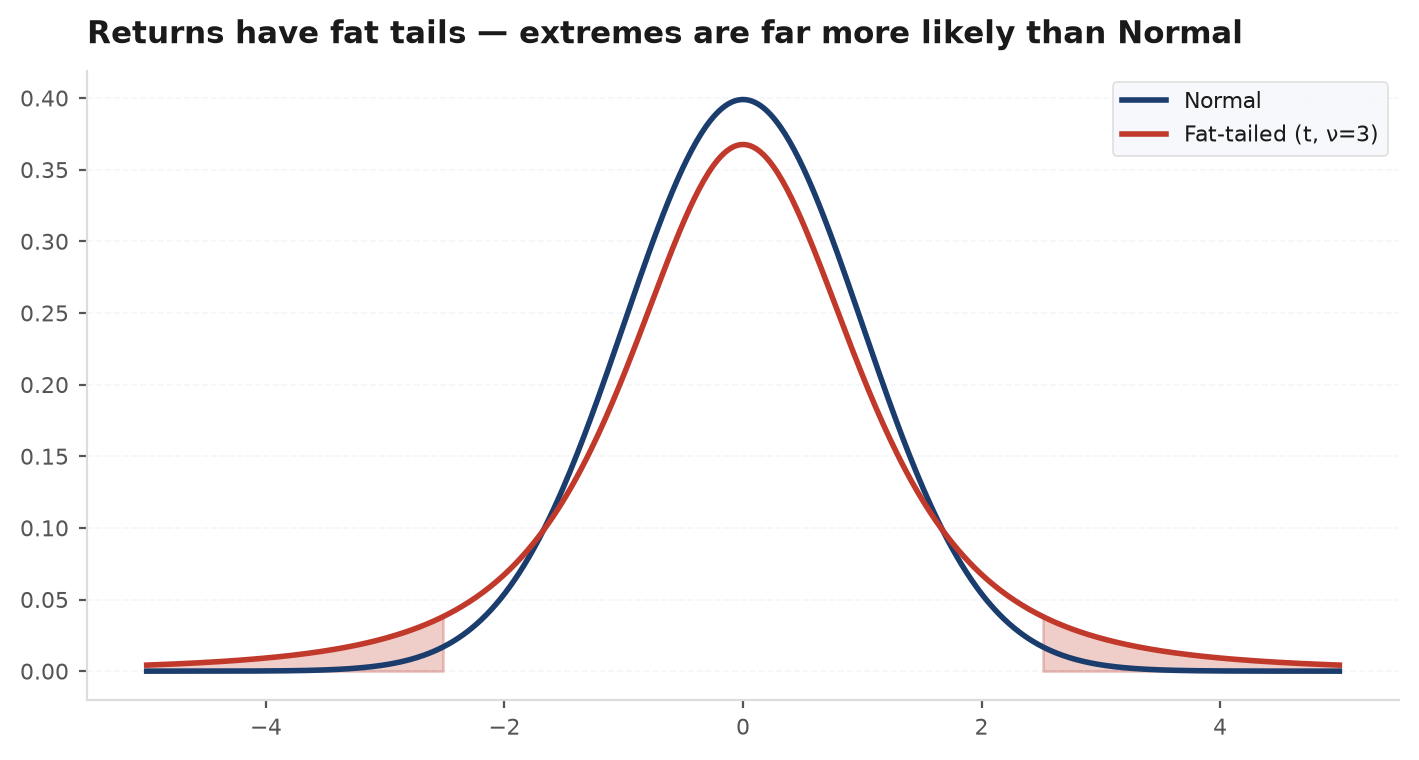
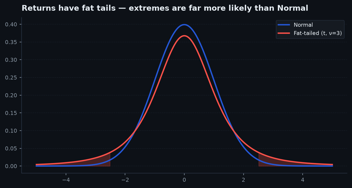
T = \frac{Z}{V / ν}, Z \sim N (0, 1), V \sim χ_{ν}^{2} independent .

Dividing by a scale estimate that is occasionally small fattens the tails: the density decays polynomially, like $∣ t ∣^{- (ν + 1)}$ , not exponentially. Moments exist only up to order $ν - 1$ : the variance is $ν / (ν - 2)$ for $ν > 2$ and infinite at $ν = 2$ ; at $ν = 1$ (the Cauchy) even the mean fails. As $ν \to \infty$ the t becomes the normal. Daily equity returns fit a t with $ν \approx 3$ – $5$ far better than a normal — the fact driving the fat-tail warnings throughout the applied course.

A normal density overlaid with a fat-tailed Student-t density on a log scale, showing the t's tails sitting far above the normal's — Normal vs Student-t tails. On the log scale the normal plunges quadratically while the t decays polynomially: events the Gaussian calls once-in-a-universe are routine under the t. Return data votes for the t.

Chi-square and F#

The Chi-square $χ_{k}^{2} = Z_{1}^{2} + \dots + Z_{k}^{2}$ (squared standard normals) is Gamma $(k /2, 1/2)$ , with $E [χ_{k}^{2}] = k$ (each $E [Z_{i}^{2}] = 1$ ) and $Var (χ_{k}^{2}) = 2 k$ (each square contributes $E [Z^{4}] - 1 = 2$ ); it is the sampling distribution of the sample variance under normality. The F distribution $F = (χ_{d_{1}}^{2} / d_{1}) / (χ_{d_{2}}^{2} / d_{2})$ compares variances — the testing distribution of Hypothesis tests and Regression & Gauss-Markov; note $t_{ν}^{2} = F_{1, ν}$ .

Pareto and power laws#

The Pareto $(α, x_{m})$ has survival function $P (X > x) = (x_{m} / x)^{α}$ , a pure power law. The $k$ -th moment:

E [X^{k}] = \int_{x_{m}}^{\infty} x^{k} α x_{m}^{α} x^{- α - 1} d x \propto \int_{x_{m}}^{\infty} x^{k - α - 1} d x, finite ⟺ k < α .

Moments simply stop existing above the tail index: $α = 1.5$ gives a mean but infinite variance — sample averages converge, sample variances never settle, and the CLT fails (see LLN & CLT). Tail indices around 3–4 for equity returns and near 1 for wealth are why extreme value theory exists: the largest observation in a power-law sample is the same order as the sum.

The relationship map#

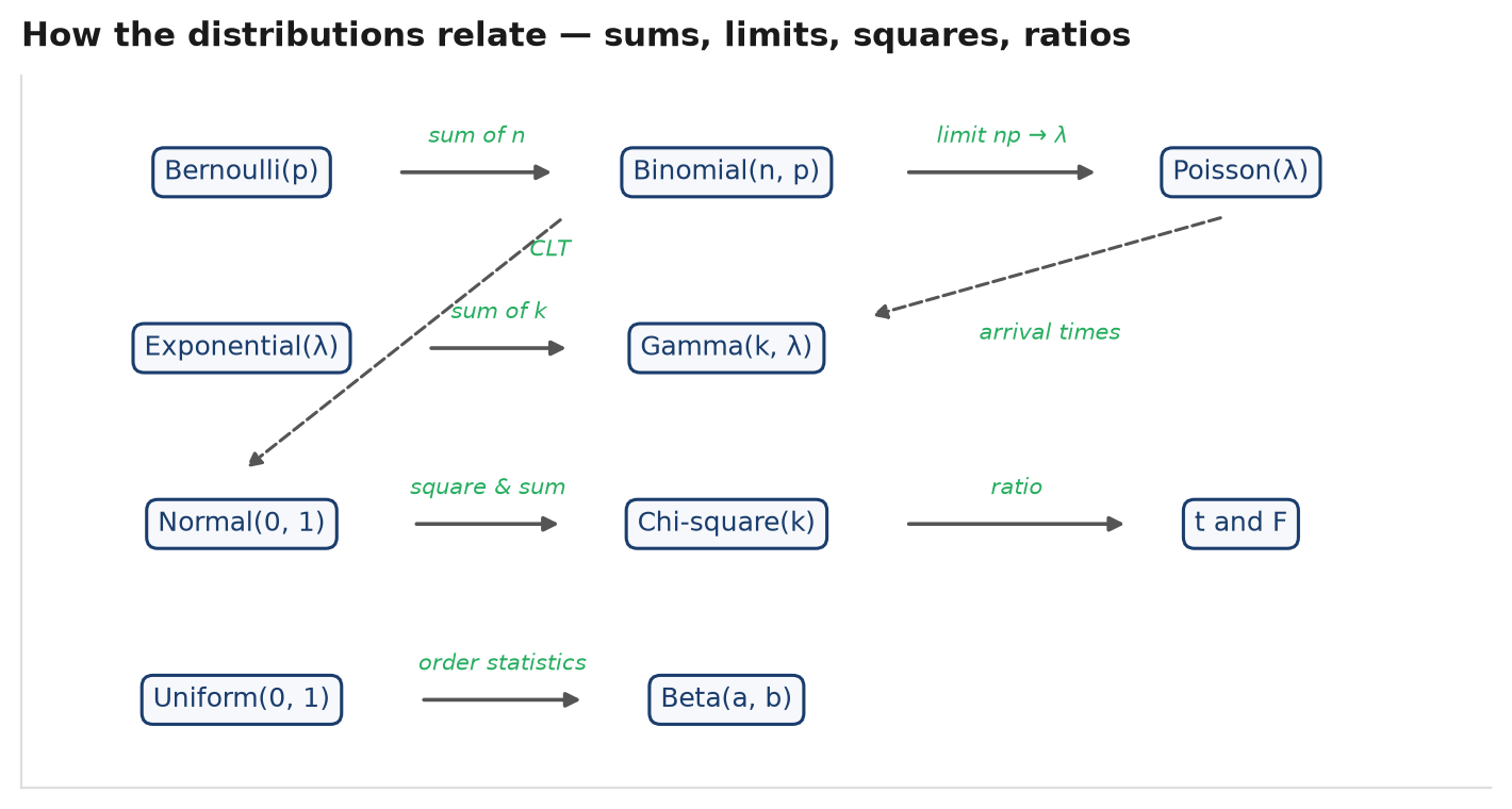
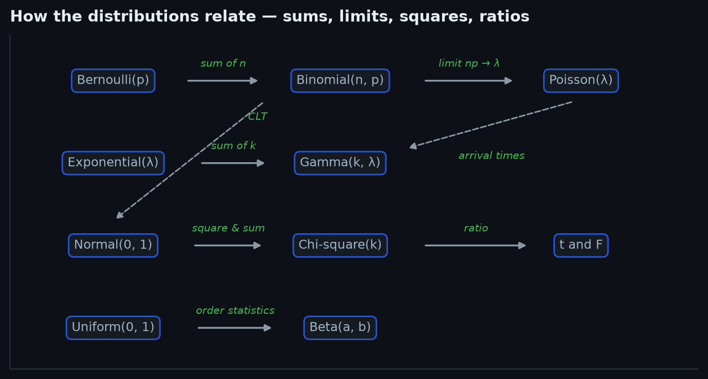
The zoo is a family tree, and the classic problems ask you to walk its edges. Bernoulli trials aggregate into the Binomial; waiting inside the same trials gives the Geometric and Negative binomial; removing replacement gives the Hypergeometric. Push $n \to \infty$ with $n p$ fixed and the Binomial becomes the Poisson; let time flow continuously and the Geometric becomes the Exponential, whose sums are Gamma, whose event counts are Poisson — the two faces of the Poisson process. Every finite-variance sum drifts to the Normal; exponentiating gives the Lognormal; squared normals sum to the Chi-square; a normal over a chi-square’s root is the Student-t; two chi-squares in ratio give the F. Uniform order statistics are Betas, and Beta(1,1) closes the loop.

A directed graph connecting the named distributions: Bernoulli to Binomial to Poisson and Normal, Geometric to Exponential to Gamma, normals to Chi-square, Student-t and F, uniforms to Beta — The family tree. Arrows are limits (Binomial to Poisson, everything to Normal), sums (Exponential to Gamma, squared normals to Chi-square), and transformations (Normal to Lognormal, ratios to t and F). Knowing the edges means never re-deriving from scratch.

The zoo at a glance#

Distribution	Support	Mean	Variance	Shows up as
Bernoulli(p)	{0, 1}	$p$	$p (1 - p)$	one trade: win or lose
Binomial(n, p)	0..n	$n p$	$n p (1 - p)$	wins in n trades; binomial tree
Geometric(p)	1, 2, ...	$1/ p$	$(1 - p) / p^{2}$	trades until first win; streaks
Neg. binomial(r, p)	r, r+1, ...	$r / p$	$r (1 - p) / p^{2}$	overdispersed counts
Hypergeometric	0..n	$n K / N$	binomial × FPC	sampling w/o replacement
Poisson(λ)	0, 1, ...	$λ$	$λ$	order arrivals, jumps, defaults
Uniform(a, b)	[a, b]	$(a + b) /2$	$(b - a)^{2} /12$	source of all simulation
Exponential(λ)	[0, ∞)	$1/ λ$	$1/ λ^{2}$	time to next order / jump
Gamma(k, λ)	[0, ∞)	$k / λ$	$k / λ^{2}$	time to k-th arrival
Beta(α, β)	[0, 1]	$α / (α + β)$	see text	win-rate posterior; order stats
Normal(μ, σ²)	ℝ	$μ$	$σ^{2}$	CLT limit of everything
Lognormal(μ, σ²)	(0, ∞)	$e^{μ + σ^{2} /2}$	see text	prices under GBM
Student-t(ν)	ℝ	$0 (ν > 1)$	$ν / (ν - 2)$	daily returns (ν ≈ 3–5)
Chi-square(k)	[0, ∞)	$k$	$2 k$	sample variance under normality
F(d₁, d₂)	[0, ∞)	$d_{2} / (d_{2} - 2)$	see text	variance ratios, regression F-tests
Pareto(α)	[xₘ, ∞)	$\frac{α x _{m}}{α - 1} (α > 1)$	∞ if α ≤ 2	tail risk, wealth, drawdowns

A seeded simulation confirms three headline claims — the Poisson limit, the summed-rate minimum of exponentials, and the Lognormal mean/median split:

zoo_checks.py

import numpy as np

rng = np.random.default_rng(11)
n_sims = 200_000

# 1) Binomial(200, 0.015) vs Poisson(3): P(X <= 1)
binom = rng.binomial(200, 0.015, n_sims)
pois = rng.poisson(3.0, n_sims)
print((binom <= 1).mean(), (pois <= 1).mean())   # 0.1961  0.1990  (exact: 0.1963, 0.1991)

# 2) min of Exp(1), Exp(2), Exp(3)  ~  Exp(6); P(the Exp(3) clock wins) = 3/6
e = rng.exponential(1.0 / np.array([1.0, 2.0, 3.0]), size=(n_sims, 3))
print(e.min(axis=1).mean(), (e.argmin(axis=1) == 2).mean())   # ~0.1667 (=1/6), ~0.500

# 3) Lognormal mu=0, sigma=0.8: mean e^{0.32}=1.377 vs median e^0=1
s = rng.lognormal(0.0, 0.8, n_sims)
print(s.mean(), np.median(s))   # ~1.377, ~1.000 — the mean/median wedge is real

→Quant lens — the zoo is a menu of nulls

Every distribution here is a null hypothesis a desk actually uses. Trade wins: Binomial — a 7-loss streak in 100 trades at a 55% win rate is expected, not a broken strategy. Order arrivals and jumps: Poisson — clustering beyond Poisson variance is signal, not noise. Prices: Lognormal — the median path lags the mean by

e^{σ^{2} /2}

. Returns: Student-t — a “6-sigma” day is a parameter error, not a market miracle. Choosing the wrong animal is the most common silent modelling error in backtesting; the gauntlet exists to catch it.

Practice problems#

→Problem 1 — Minimum of exponentials

Three servers fail after independent Exponential times with rates 1, 2, and 3 per year. What is the law of the time to first failure, and the probability the rate-3 server fails first?

Solution. Survival functions multiply for a minimum of independent variables:

P (min > t) = e^{- t} \cdot e^{- 2 t} \cdot e^{- 3 t} = e^{- 6 t} ⟹ min \sim Exp (6), E [min] = \frac{1}{6} year .

For the race, each clock wins in proportion to its rate: $P (rate-3 first) = 3/ (1 + 2 + 3) = 1/2$ , from $P (X_{1} < X_{2}) = \int_{0}^{\infty} λ_{1} e^{- λ_{1} t} e^{- λ_{2} t} d t = λ_{1} / (λ_{1} + λ_{2})$ with clocks 1 and 2 grouped into one Exp(3) competitor. The encore: after the first failure, memorylessness restarts the survivors fresh.

→Problem 2 — Sum and conditional of Poissons

Buy orders arrive Poisson(2) per second and sell orders Poisson(3), independently. What is the distribution of total orders per second? Given exactly 10 orders arrived, how many were buys?

Solution. MGFs multiply: $e^{2 (e^{t} - 1)} \cdot e^{3 (e^{t} - 1)} = e^{5 (e^{t} - 1)}$ , so the total is Poisson(5). For the conditional, compute directly with $B \sim Poi (2)$ , $S \sim Poi (3)$ :

P (B = k ∣ B + S = 10) = \frac{e ^{- 2} \frac{2 ^{k}}{k !} \cdot e ^{- 3} \frac{3 ^{10 - k}}{( 10 - k )!}}{e ^{- 5} \frac{5 ^{10}}{10 !}} = (k 10) (\frac{2}{5})^{k} (\frac{3}{5})^{10 - k} .

Binomial(10, 2/5) — given the total, each arrival is independently a buy with probability $λ_{B} / (λ_{B} + λ_{S})$ : the splitting/thinning duality, the workhorse of Poisson processes.

→Problem 3 — Normal conditional probability

A stock’s annual return is $N (8%, 20 %^{2})$ . Given the year is positive, what is the probability it exceeds 20%?

Solution. Standardise: $P (R > 0) = Φ (0.4) \approx 0.6554$ , $P (R > 0.20) = 1 - Φ (0.6) \approx 0.2743$ . Since ${R > 0.20} \subset {R > 0}$ ,

P (R > 0.20 ∣ R > 0) = \frac{P ( R > 0.20 )}{P ( R > 0 )} \approx \frac{0.2743}{0.6554} \approx 0.42.

The trap is reaching for a joint density — nested events need only a ratio. A common follow-up is the truncated mean via the inverse Mills ratio: $E [R ∣ R > 0] = μ + σ φ (z_{0}) /Φ (- z_{0}) \approx 19.2%$ with $z_{0} = - μ / σ = - 0.4$ .

→Problem 4 — Which distribution models it?

Rapid-fire: (a) days until your strategy’s first losing day; (b) defaults this year in a book of 500 loans; (c) a stock price in one year under constant vol; (d) the largest of 20 independent uniform bids; (e) daily P&L of a strategy with occasional violent losses.

Solution.(a) Geometric — memorylessness says a winning streak does not make a loss “due”. (b) Binomial(500, $p$ ), collapsing to Poisson( $500 p$ ) — the law of rare events. (c) Lognormal — GBM exponentiates a normal. (d) Beta: the max of 20 uniforms is Beta(20, 1) with $E = 20/21$ . (e) Student-t with low $ν$ — polynomial tails, finite mean. The grading key is the mechanism: trials, rare counts, multiplicative growth, order statistics, fat tails.

→Problem 5 — Lognormal mean vs median (the vol-drag trap)

Log returns are $N (0, 0. 8^{2})$ , so the price relative is $S = e^{X}$ with $E [S] = e^{0.32} \approx 1.377$ — up 38%. Should a holder expect to make money?

Solution. No — the median outcome is $e^{0} = 1$ : half of all paths finish flat or down, despite a +38% mean. The wedge is Jensen’s inequality on the convex map $x \mapsto e^{x}$ :

E [e^{X}] = e^{μ + σ^{2} /2} > e^{μ} = e^{median (X)} = median (e^{X}),

using that the median commutes with monotone maps while the mean does not: a few explosive paths carry the entire mean. This is volatility drag in distributional form — the median compound outcome grows at $μ - σ^{2} /2$ in GBM terms, so headline expected returns on high-variance assets overstate what the median holder gets. The inequality machinery arrives in Inequalities & tail bounds.

Next: portfolios live and die by how variables move together — joint densities, correlation, the bivariate normal, and conditional expectation as the best predictor. Joint distributions & correlation.