Joint distributions & correlation

One random variable describes a coin; markets are thousands of coins flipped together, and everything that matters — diversification, hedging, factor exposure, contagion — lives in how they co-move. This chapter builds the machinery of joint behaviour: joint and conditional densities, convolution, covariance and its Cauchy–Schwarz bound, the bivariate normal whose conditional mean is the regression line, and conditional expectation as the provably best predictor, with the tower property and the law of total variance as its calculus.

✦Intuition — the joint distribution is where portfolios live

Marginals are the biographies of individual assets; the joint distribution is the story of the whole market. Two portfolios can hold assets with identicalmarginal distributions and have wildly different risk: if the pieces move together, the diversification you thought you bought does not exist. Every question of the form “what should I expect for Y, having seen X?” — the primal question of forecasting — is a question about a conditional distribution. And the single most-used regression in finance, beta against the market, will fall out of this chapter as a two-line consequence of the bivariate normal.

Joint, marginal, conditional#

For two discrete variables the joint pmf is $p (x, y) = P (X = x, Y = y)$ ; for continuous variables the joint density $f (x, y)$ assigns probability $\iint_{A} f$ to a region $A$ . Marginals come from summing or integrating the partner out, and conditionals from dividing:

f_{X} (x) = \int f (x, y) d y, f_{Y ∣ X} (y ∣ x) = \frac{f ( x , y )}{f _{X} ( x )} .

The conditional density is a genuine density in $y$ for each fixed $x$ — renormalised by the marginal so it integrates to one. Independence is the special case where conditioning changes nothing, which is equivalent to factorisation:

X ⊥ Y ⟺ f (x, y) = f_{X} (x) f_{Y} (y) for all x, y ⟺ f_{Y ∣ X} (y ∣ x) = f_{Y} (y) .

Worked example. A two-asset market has joint pmf for (stock up/down, bond up/down):

	Bond up	Bond down	Marginal (stock)
Stock up	0.15	0.35	0.50
Stock down	0.30	0.20	0.50
Marginal (bond)	0.45	0.55	1.00

Marginally, stock and bond are near coin-flips. But $P (bond up ∣ stock down) = 0.30/0.50 = 0.60$ versus the unconditional 0.45 — bonds rally when stocks fall. Independence fails because $0.15 \neq = 0.50 \times 0.45 = 0.225$ . This flight-to-quality asymmetry is exactly the information a joint distribution carries and marginals discard — and it is the entire basis of the 60/40 portfolio.

Convolution — the distribution of a sum#

If $X ⊥ Y$ , the density of $S = X + Y$ is the convolution: condition on $X = x$ , note $S = s$ requires $Y = s - x$ , and integrate over the ways:

f_{S} (s) = \int_{- \infty}^{\infty} f_{X} (x) f_{Y} (s - x) d x .

✦Derivation — sum of two uniforms is a triangle

Let $X, Y \sim Unif (0, 1)$ independent. The integrand is 1 exactly when $0 \leq x \leq 1$ and $0 \leq s - x \leq 1$ , i.e. $max (0, s - 1) \leq x \leq min (1, s)$ . The length of that interval is

f_{S} (s) = {s 2 - s 0 \leq s \leq 1 1 < s \leq 2

— the triangular density peaking at 1. One convolution already begins the march toward the bell: corners smooth, mass concentrates in the middle. Convolve again (three uniforms) and you get piecewise parabolas hugging a normal — the CLT of LLN & the CLT visibly at work.

For normals, convolution is best done with MGFs (derived in the distribution zoo): independent $N (μ_{1}, σ_{1}^{2})$ and $N (μ_{2}, σ_{2}^{2})$ have MGF product $e^{(μ_{1} + μ_{2}) t + (σ_{1}^{2} + σ_{2}^{2}) t^{2} /2}$ , so the sum is $N (μ_{1} + μ_{2}, σ_{1}^{2} + σ_{2}^{2})$ . Means add; for independent variables, variances add. Correlation is precisely what breaks that second rule.

Covariance and correlation#

Covariance measures linear co-movement:

Cov (X, Y) = E [(X - μ_{X}) (Y - μ_{Y})] = E [X Y] - μ_{X} μ_{Y} .

It is symmetric, bilinear ( $Cov (a X + b Z, Y) = a Cov (X, Y) + b Cov (Z, Y)$ ), equals the variance on the diagonal, and vanishes under independence (because $E [X Y] = E [X] E [Y]$ factorises). The variance of a sum picks up a cross term:

Var (X + Y) = Var (X) + Var (Y) + 2 Cov (X, Y) .

Correlation is covariance made scale-free, $ρ = Cov (X, Y) / (σ_{X} σ_{Y})$ , and it is trapped in $[- 1, 1]$ by Cauchy–Schwarz:

✦Proof — Cauchy–Schwarz, hence |ρ| ≤ 1

For any random variables $U, V$ with finite second moments and any real $t$ ,

0 \leq E [(U - t V)^{2}] = E [U^{2}] - 2 t E [U V] + t^{2} E [V^{2}] .

A quadratic in $t$ that never goes negative must have non-positive discriminant: $4 E [U V]^{2} - 4 E [U^{2}] E [V^{2}] \leq 0$ , i.e. $E [U V]^{2} \leq E [U^{2}] E [V^{2}]$ . Apply this to the centred variables $U = X - μ_{X}$ , $V = Y - μ_{Y}$ to get $Cov (X, Y)^{2} \leq σ_{X}^{2} σ_{Y}^{2}$ , hence $∣ ρ ∣ \leq 1$ . Equality holds iff $E [(U - t V)^{2}] = 0$ for some $t$ — iff $Y$ is an exact linear function of $X$ . $■$

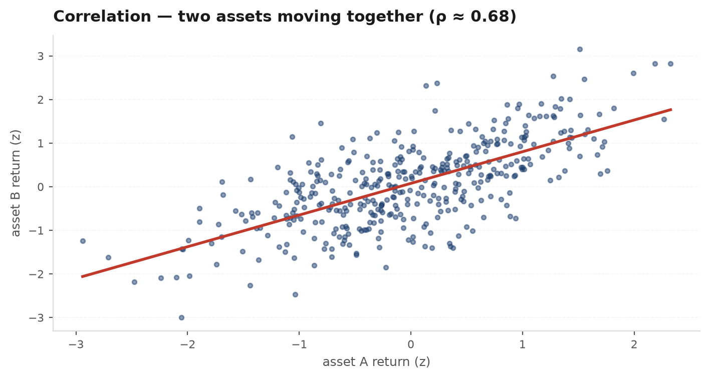
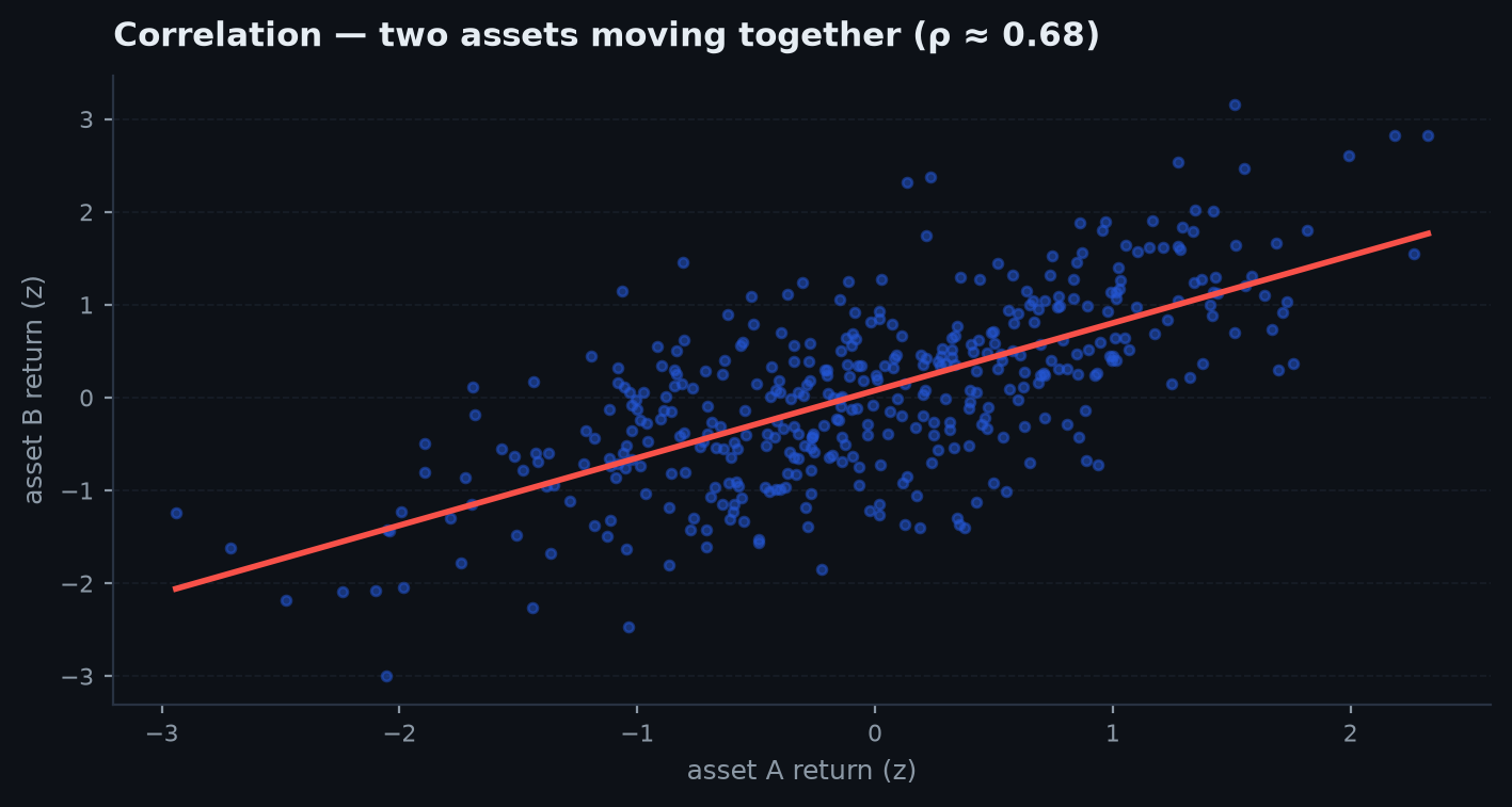
Zero correlation is not independence. The canonical counterexample: let $X \sim N (0, 1)$ and $Y = X^{2}$ . Then $Cov (X, Y) = E [X^{3}] - E [X] E [X^{2}] = 0$ by symmetry (odd moments of a symmetric law vanish), yet $Y$ is a deterministic function of $X$ — maximal dependence, zero correlation. Correlation sees only the linear shadow of dependence. Markets exploit the gap: index returns and index volatility are nearly uncorrelated in sign yet fiercely dependent — the leverage effect that copulas exist to capture.

Scatter plots of paired data at several correlation levels, from strongly negative through zero to strongly positive — What correlation looks like in a scatter. But beware the converse: a symmetric U-shaped cloud has zero correlation and total dependence. The coefficient measures linear association only.

The bivariate normal#

The bivariate normal is the joint law of two Gaussians glued together with a single dependence parameter $ρ$ :

f (x, y) = \frac{1}{2 π σ _{X} σ _{Y} 1 - ρ ^{2}} exp [- \frac{1}{2 ( 1 - ρ ^{2} )} (z_{X}^{2} - 2 ρ z_{X} z_{Y} + z_{Y}^{2})],

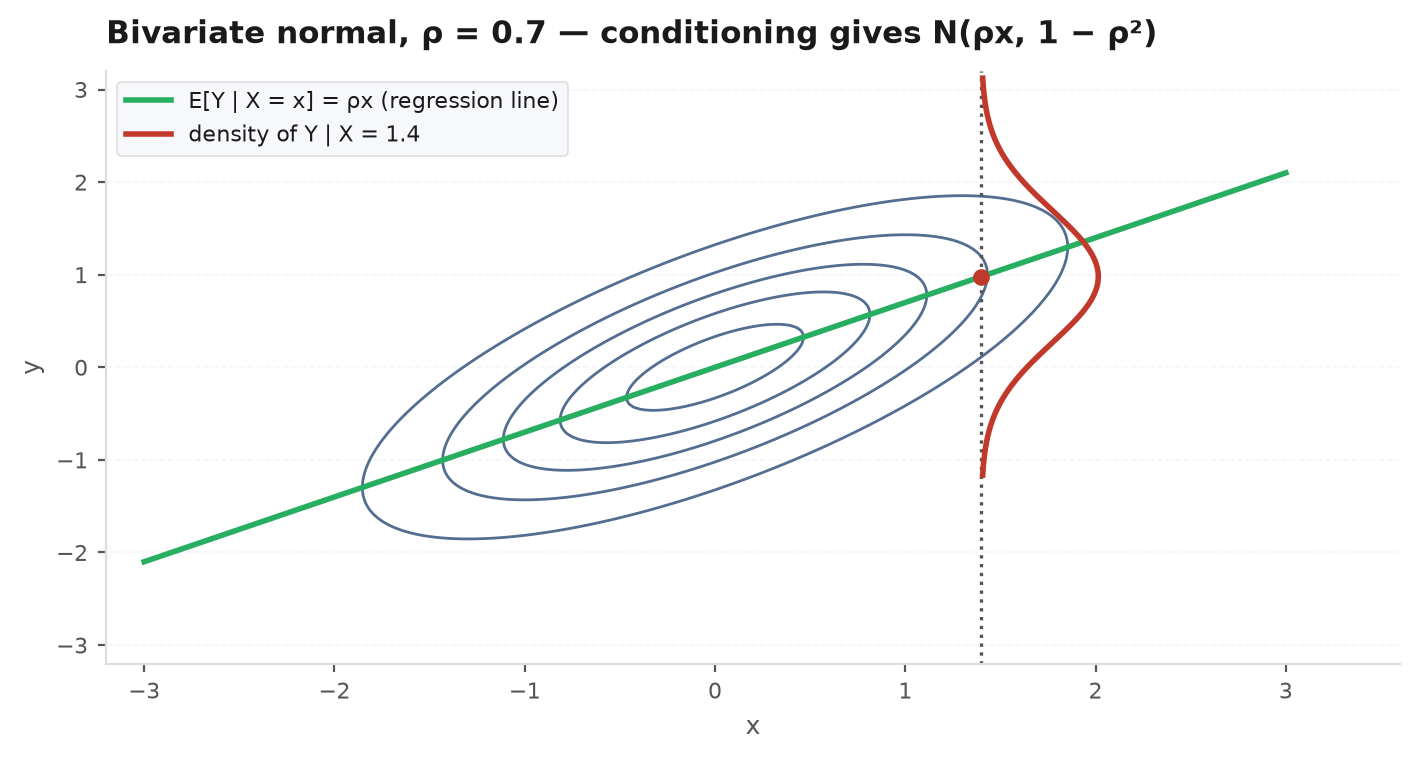
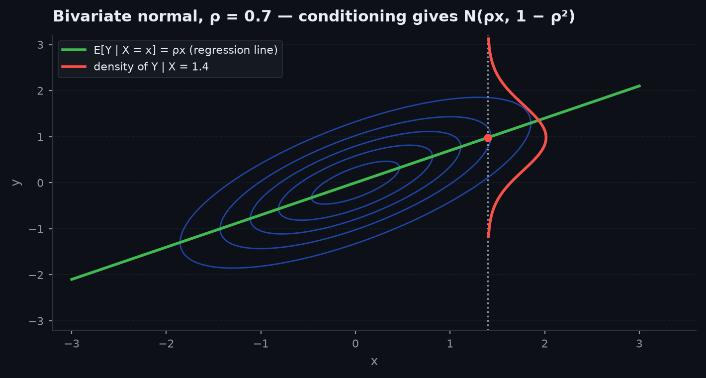
with $z_{X} = (x - μ_{X}) / σ_{X}$ , $z_{Y} = (y - μ_{Y}) / σ_{Y}$ . Its contours are ellipses tilted by correlation, and its conditional distribution is the most important calculation in applied statistics:

✦Derivation — the conditional law, and the regression line falls out

Fix $x$ and view the exponent as a function of $z_{Y}$ . Complete the square:

z_{X}^{2} - 2 ρ z_{X} z_{Y} + z_{Y}^{2} = (z_{Y} - ρ z_{X})^{2} + (1 - ρ^{2}) z_{X}^{2},

so, after dividing by the marginal of $X$ (which absorbs the $(1 - ρ^{2}) z_{X}^{2}$ piece), the conditional density of $Y$ given $X = x$ is proportional to $exp [- (z_{Y} - ρ z_{X})^{2} / (2 (1 - ρ^{2}))]$ — again normal:

Y ∣ X = x \sim N (μ_{Y} + ρ \frac{σ _{Y}}{σ _{X}} (x - μ_{X}), σ_{Y}^{2} (1 - ρ^{2})) .

Read it slowly, because three classical facts are hiding in it. (1) The conditional mean is linear in $x$ with slope $β = ρ σ_{Y} / σ_{X} = Cov (X, Y) / Var (X)$ — the OLS regression coefficient of Regression & Gauss-Markov and the market beta of factor models, derived rather than assumed. (2) The conditional variance $σ_{Y}^{2} (1 - ρ^{2})$ does not depend on $x$ — knowing $X$ removes exactly the fraction $ρ^{2}$ of the variance, which is why $R^{2} = ρ^{2}$ in simple regression. (3) Because the slope multiplies $ρ < 1$ , extreme $x$ predicts a less extreme $y$ — regression to the mean, as a theorem.

Elliptical contours of a bivariate normal density with the conditional mean line drawn through them, flatter than the 45-degree axis of the ellipse — Bivariate normal contours with the regression line E[Y|X=x]. Note the line is flatter than the ellipse’s major axis — the geometric face of regression to the mean: best predictions shrink toward the mean by the factor rho.

Worked example. A stock and the index have annual returns that are bivariate normal with $μ_{S} = 12%, σ_{S} = 30%$ , $μ_{M} = 8%, σ_{M} = 18%$ , $ρ = 0.6$ . Given the index falls 10%, the stock’s conditional distribution has mean $0.12 + 0.6 \cdot \frac{0.30}{0.18} (- 0.10 - 0.08) = 0.12 - 0.18 = - 6%$ and standard deviation $0.30 1 - 0.36 = 24%$ . The slope $0.6 \times 0.30/0.18 = 1.0$ is the stock’s beta; the residual 24% is its idiosyncratic risk.

A Gaussian privilege. For jointly normal variables, $ρ$ is the entire dependence structure — zero correlation implies full independence (the joint density factorises when $ρ = 0$ ). For every other family, correlation is a one-number summary of something richer, and tail dependence can hide behind modest $ρ$ . Assuming Gaussian dependence for assets whose crashes are synchronised is the modelling error behind 2008’s copula disasters — see Copulas & dependence.

The multivariate normal $X \sim N (μ, Σ)$ generalises: it is defined by the property that every linear combination $a^{⊤} X$ is univariate normal, with mean $a^{⊤} μ$ and variance $a^{⊤} Σ a$ . That last expression forces $Σ$ to be positive semi-definite: it is a variance, and variances cannot be negative — so $a^{⊤} Σ a \geq 0$ for every $a$ by construction, which is why a “correlation matrix” you invent by hand can fail to correspond to any possible world (and why estimated covariance matrices need care). Portfolio variance is the special case $a = w$ , the vector of weights.

Conditional expectation — the best predictor#

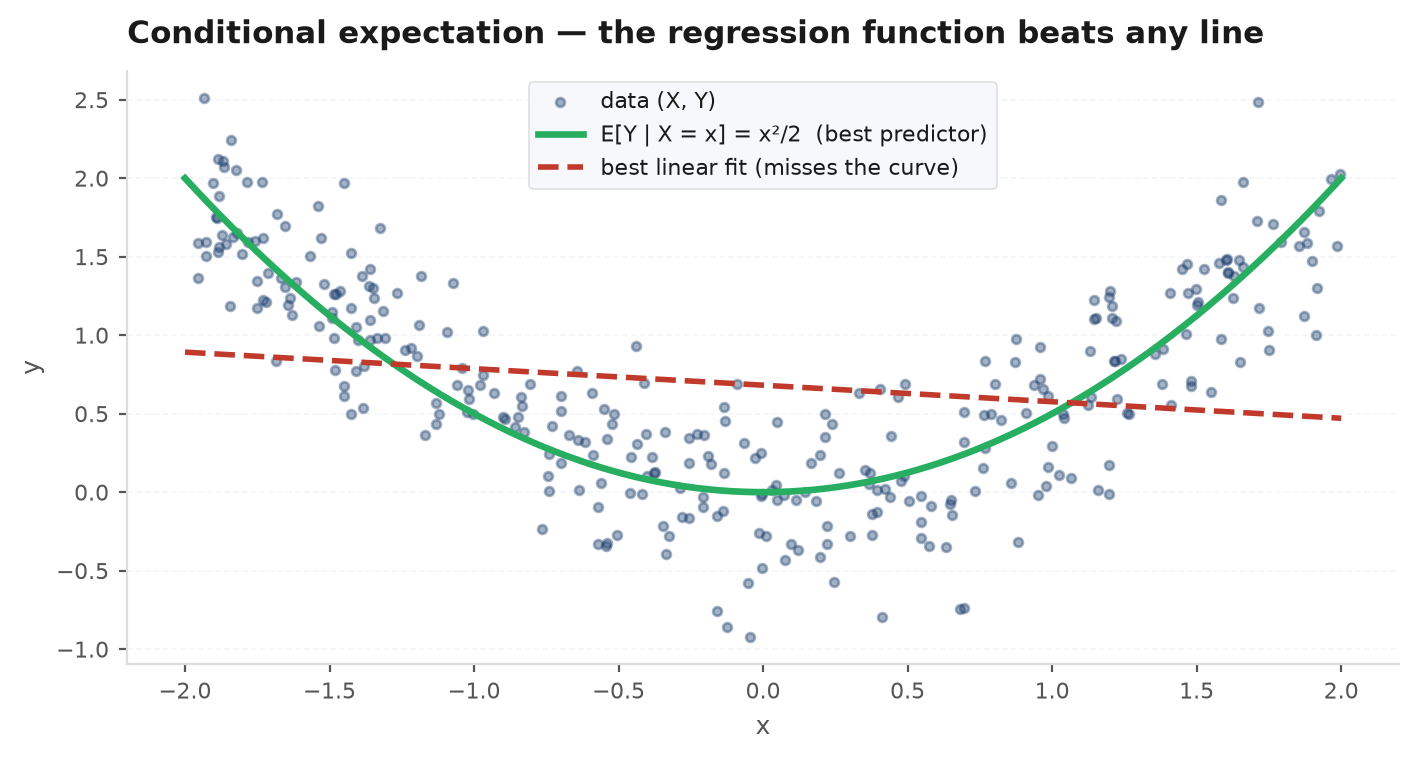
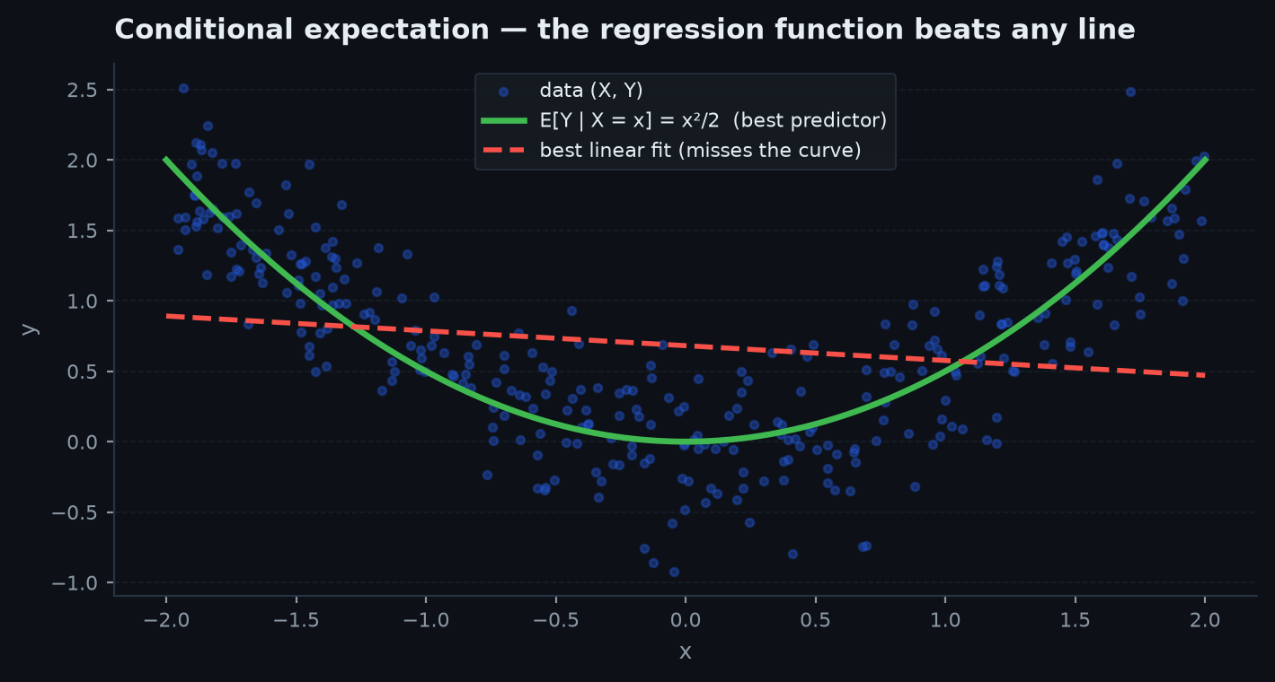
$E [Y ∣ X]$ is a random variable — a function of $X$ that answers “what is my best guess of $Y$ once I see $X$ ?” And “best” is a theorem, not a slogan:

✦Proof — E[Y|X] minimises mean squared error

Let $g (X)$ be any predictor and write $m (X) = E [Y ∣ X]$ . Decompose:

E [(Y - g (X))^{2}] = E [(Y - m (X))^{2}] + E [(m (X) - g (X))^{2}] + 2 E [(Y - m (X)) (m (X) - g (X))] .

The cross term dies by conditioning: given $X$ , the factor $m (X) - g (X)$ is a constant and $E [Y - m (X) ∣ X] = 0$ by definition of $m$ ; the tower property below then kills the unconditional expectation too. What remains is minimised by choosing $g = m$ , and the minimum MSE is the leftover $E [Var (Y ∣ X)]$ . $■$ Every forecasting model — OLS, trees, neural networks — is an attempt to approximate this one object with finite data.

✦Proof — the tower property (discrete case)

Claim: $E [E [Y ∣ X]] = E [Y]$ . Expand the outer expectation over the values of $X$ :

x \sum P (X = x) y \sum y P (Y = y ∣ X = x) = y \sum y x \sum P (Y = y ∣ X = x) P (X = x) = y \sum y P (Y = y) = E [Y],

where the inner step is the law of total probability from Axioms, conditioning & Bayes. Averaging your conditional forecasts over what you might observe returns your unconditional forecast — you cannot expect to change your expectation. (This “no free updates” principle becomes the martingale property in Martingales & optional stopping.) $■$

Variance decomposes the same way — the law of total variance(“Adam & Eve”, Eve for E-V-E):

Var (Y) = E [Var (Y ∣ X)] + Var (E [Y ∣ X]) .

✦Derivation — Adam & Eve in three lines

Start from $Var (Y) = E [Y^{2}] - E [Y]^{2}$ and hit each term with the tower property: $E [Y^{2}] = E [Var (Y ∣ X) + E [Y ∣ X]^{2}]$ (the conditional version of the same identity), and $E [Y]^{2} = (E E [Y ∣ X])^{2}$ . Subtract:

Var (Y) = E [Var (Y ∣ X)] + (E [E [Y ∣ X]^{2}] - (E E [Y ∣ X])^{2}) = E [Var (Y ∣ X)] + Var (E [Y ∣ X]) . ■

Total risk = average within-scenario risk + between-scenariorisk. For a strategy whose P&L depends on a hidden regime, the second term is regime risk — invisible in any single regime’s backtest, and the reason regime detection matters.

A scatter of Y against X with the conditional mean curve overlaid, and vertical slices showing the conditional distribution of Y at several values of X — Conditional expectation as a curve through vertical slices: at each x, average the Y values in the slice. The curve minimises mean squared error among all functions of X; the scatter around it is E[Var(Y|X)], the irreducible noise.

A closing definition worth a mention: variables are exchangeable if their joint law is invariant under permutations — weaker than iid (exchangeable variables can be correlated, like draws without replacement) yet strong enough to power symmetry arguments: any of $n$ exchangeable variables is the maximum with probability exactly $1/ n$ . De Finetti’s theorem says exchangeable sequences are mixtures of iid ones — the philosophical bedrock of Bayesian inference.

A seeded simulation verifies the two headline formulas — the bivariate-normal conditional law and Adam & Eve:

joint_checks.py

import numpy as np

rng = np.random.default_rng(11)
n = 500_000

# Bivariate normal: stock (12%, 30%), index (8%, 18%), rho = 0.6
mu_s, sig_s, mu_m, sig_m, rho = 0.12, 0.30, 0.08, 0.18, 0.6
z1, z2 = rng.standard_normal(n), rng.standard_normal(n)
m = mu_m + sig_m * z1                                   # index return
s = mu_s + sig_s * (rho * z1 + np.sqrt(1 - rho**2) * z2)  # stock return

# Conditional law given index ~ -10%: theory mean -6%, sd 24%
sl = (m > -0.105) & (m < -0.095)
print(s[sl].mean(), s[sl].std())        # ~ -0.060, ~0.240

# Adam & Eve: Var(S) = E[Var(S|M)] + Var(E[S|M])
within = (1 - rho**2) * sig_s**2        # 0.0576
between = (rho * sig_s / sig_m)**2 * sig_m**2  # beta^2 * Var(M) = 0.0324
print(s.var(), within + between)        # both ~0.0900 = 0.30^2

→Quant lens — diversification is a statement about the joint distribution

For an equal-weight portfolio of

n

assets, each with variance

σ^{2}

and pairwise correlation

ρ

, the portfolio variance is

\frac{σ ^{2}}{n} + \frac{n - 1}{n} ρ σ^{2} \to ρ σ^{2}

. The idiosyncratic term dies at rate

1/ n

; the correlated term never dies. Diversification eliminates only the independent part of risk, and its limit is set entirely by the average correlation — which is why portfolios that look diversified in calm markets (low

ρ

) concentrate violently in crises, when correlations lurch toward one. Risk budgets built off the joint distribution, not a stack of marginals, are the subject of Portfolio construction and Risk management.

Practice problems#

→Problem 1 — E[X | X + Y]

$X, Y$ are iid with finite mean. Find $E [X ∣ X + Y = s]$ .

Solution. By symmetry (exchangeability), $X$ and $Y$ have identical conditional laws given the sum, so $E [X ∣ S] = E [Y ∣ S]$ . But linearity forces $E [X ∣ S] + E [Y ∣ S] = E [X + Y ∣ S] = S$ . Therefore

E [X ∣ X + Y = s] = \frac{s}{2},

with no distribution needed — an answer you should be able to give in one breath. Generalisation: for $n$ iid terms, $E [X_{1} ∣ \sum_{i = 1}^{n} X_{i} = s] = s / n$ . The grinding alternative (write the joint density, condition, integrate) takes ten minutes and works only for named distributions; symmetry works for all of them.

→Problem 2 — Correlation of X and X + Y

$X, Y$ are iid with variance $σ^{2}$ . Find $Corr (X, X + Y)$ .

Solution. Bilinearity: $Cov (X, X + Y) = Var (X) + Cov (X, Y) = σ^{2} + 0$ . The scales: $σ_{X} = σ$ , $σ_{X + Y} = σ 2$ . So

Corr (X, X + Y) = \frac{σ ^{2}}{σ \cdot σ 2} = \frac{1}{2} \approx 0.707.

The natural follow-up: with $n$ terms, $Corr (X_{1}, \sum_{1}^{n} X_{i}) = 1/ n$ . This is why a single asset correlates $1/ n$ with an equal-weight basket containing it, and why an index component can look “highly correlated with the market” on no signal at all — a trap in naive alpha attribution.

→Problem 3 — Sum of n dice, given the first

Roll five fair dice. The first shows a 6. What is the expected total of all five?

Solution. Independence means conditioning on the first die leaves the others untouched:

E [i = 1 \sum 5 X_{i} X_{1} = 6] = 6 + 4 \times 3.5 = 20.

The point of the question is the contrast with Problem 1: conditioning on a component shifts the expectation additively, while conditioning on the sum redistributes it symmetrically. A sharper variant: given the total of five dice is 20, the expected first die is $20/5 = 4$ by exchangeability — same machinery, opposite direction. Confusing the two directions (conditioning on parts vs wholes) is the most common error in this problem family — the gambler’s fallacy is exactly the belief that components must compensate within a fixed-sum story that nobody promised.

→Problem 4 — Joint law of the min and max of uniforms

$U_{1}, \dots, U_{n}$ are iid Unif(0,1). Find the joint density of $(m, M) = (min, max)$ , and $E [M - m]$ .

Solution. Start from the joint CDF-style event: for $x < y$ , $P (m > x, M \leq y) = P (all U_{i} \in (x, y]) = (y - x)^{n}$ . Differentiate once in $y$ and once in $x$ (with a sign for the direction of the min event):

f_{m, M} (x, y) = n (n - 1) (y - x)^{n - 2}, 0 \leq x < y \leq 1.

Marginally $M = U_{(n)}$ is Beta( $n$ , 1) with mean $n / (n + 1)$ and $m = U_{(1)}$ is Beta(1, $n$ ) with mean $1/ (n + 1)$ , so the expected range is $E [M - m] = \frac{n}{n + 1} - \frac{1}{n + 1} = \frac{n - 1}{n + 1}$ . Note min and max are positively correlated (a high min drags the max up) — independence would be the wrong instinct. The full order-statistics toolkit arrives in Order statistics & extremes.

→Problem 5 — Variance of a correlated portfolio

Two assets have volatilities 20% and 30% with correlation 0.5. You hold weights 60/40. What is the portfolio volatility? What correlation would make a 50/50 portfolio of two 20%-vol assets completely riskless?

Solution. Apply $σ_{p}^{2} = w_{1}^{2} σ_{1}^{2} + w_{2}^{2} σ_{2}^{2} + 2 w_{1} w_{2} ρ σ_{1} σ_{2}$ :

σ_{p}^{2} = 0.36 (0.04) + 0.16 (0.09) + 2 (0.6) (0.4) (0.5) (0.2) (0.3) = 0.0144 + 0.0144 + 0.0144 = 0.0432,

so $σ_{p} = 0.0432 \approx 20.8%$ — barely above the safer asset’s 20%, despite 40% of the book in the 30%-vol asset: that is diversification quantified. For the second part, set $σ_{p}^{2} = \frac{1}{4} σ^{2} + \frac{1}{4} σ^{2} + \frac{1}{2} ρ σ^{2} = \frac{σ ^{2}}{2} (1 + ρ) = 0$ — which requires $ρ = - 1$ : perfect negative correlation, i.e. an exact hedge. Cauchy–Schwarz says no joint distribution can do better, which is why a true riskless hedge requires a linear relationship — the deep reason derivatives are hedged with their underlyings and not with proxies.

Next: the conditional means computed above deserve to be first-class objects — $E [X ∣ Y]$ as a random variable in its own right, with the tower rule, the projection picture, and the variance decomposition. Conditional expectation.