Numerical methods

Most of quantitative finance has no closed form. Implied volatility is the root of an equation nobody can invert; American options have no Black-Scholes; most expectations are integrals nobody can do. What stands between the model and a number is a small set of numerical methods — root-finding, quadrature, trees, and Monte Carlo — plus the variance-reduction tricks that make Monte Carlo cheap enough to use. This chapter builds each one and races them against each other on the same option.

✦Intuition — accuracy is bought, and every method has a price list

Every numerical method converts compute into accuracy at a different exchange rate. Bisection buys one bit of accuracy per function call; Newton’s method roughly doubles the number of correct digits per call; a binomial tree’s error shrinks like $1/ n$ ; crude Monte Carlo crawls at $1/ n$ — to get one more digit you need a hundred times the paths. The craft is matching the method to the problem: fast converters when you have smoothness and derivatives, robust plodders when you have nothing, and — when you are stuck with Monte Carlo, as you usually are in high dimensions — variance reduction, which changes not the exchange rate but the constant in front of it, often by a factor of ten or more. Free accuracy, if you know the derivations.

Root-finding: bisection and Newton#

The prototype problem: find $x$ with $f (x) = 0$ . Bisection starts with a bracket $[a, b]$ where $f$ changes sign, evaluates the midpoint, keeps the half that still brackets the root, and repeats. The bracket halves each step, so the error after $k$ steps is $(b - a) / 2^{k}$ — linear convergence, one bit per evaluation, guaranteed for any continuous $f$ . Newton’s method is greedier: linearise $f$ at the current guess and jump to where the tangent line crosses zero,

x_{n + 1} = x_{n} - \frac{f ( x _{n} )}{f ^{'} ( x _{n} )} .

Near a simple root the error squares each step ( $e_{n + 1} \approx C e_{n}^{2}$ ): quadratic convergence, doubling the correct digits per iteration — three or four steps to machine precision. The price is fragility: it needs the derivative, and a bad start can diverge. Production code hybridises — Newton steps inside a bisection-maintained bracket.

→How implied_vol works

Implied volatility is exactly this problem: solve

f (σ) = BS (S, K, T, r, σ) - C_{mkt} = 0

. It is a Newton solver’s dream:

f^{'} (σ)

is vega, available in closed form, and BS price is monotonically increasing in

σ

, so the root is unique. The update is

σ_{n + 1} = σ_{n} - (BS (σ_{n}) - C_{mkt}) / vega (σ_{n})

, and edgekit’s implied_vol converges in a handful of iterations — falling back to bisection where vega collapses (deep in/out-of-the-money, short expiry), precisely the regions where Newton stalls on a flat function. See Options & greeks for what the resulting surface means.

Numerical integration#

Prices are expectations, and expectations are integrals: $E [g (X)] = \int g (x) p (x) d x$ . In one dimension, deterministic quadrature is unbeatable. The trapezoid rule joins sample points with straight lines (error $O (h^{2})$ for step $h$ ); Simpson’s rule fits parabolas through triples of points,

\int_{a}^{b} g (x) d x \approx \frac{h}{3} (g_{0} + 4 g_{1} + 2 g_{2} + 4 g_{3} + \dots + g_{n}), error O (h^{4}),

so doubling the points buys sixteen times the accuracy on smooth integrands. This is how you price a European option under any density you can evaluate — integrate payoff times density on a grid. The catch is the curse of dimensionality: a grid in $d$ dimensions needs $m^{d}$ points, hopeless for a basket of 20 assets or a path-dependent payoff over 252 steps. High dimensions belong to Monte Carlo, whose $1/ n$ rate is slow but — crucially — dimension-independent.

Binomial trees: CRR and its convergence#

Between closed forms and Monte Carlo sit trees. The Cox-Ross-Rubinstein tree chops $[0, T]$ into $n$ steps of $Δ t = T / n$ and lets the price jump up by $u$ or down by $d$ each step, with a risk-neutral up-probability $p$ chosen to match the risk-free drift and the volatility:

u = e^{σ Δ t}, d = \frac{1}{u}, p = \frac{e ^{r Δ t} - d}{u - d} .

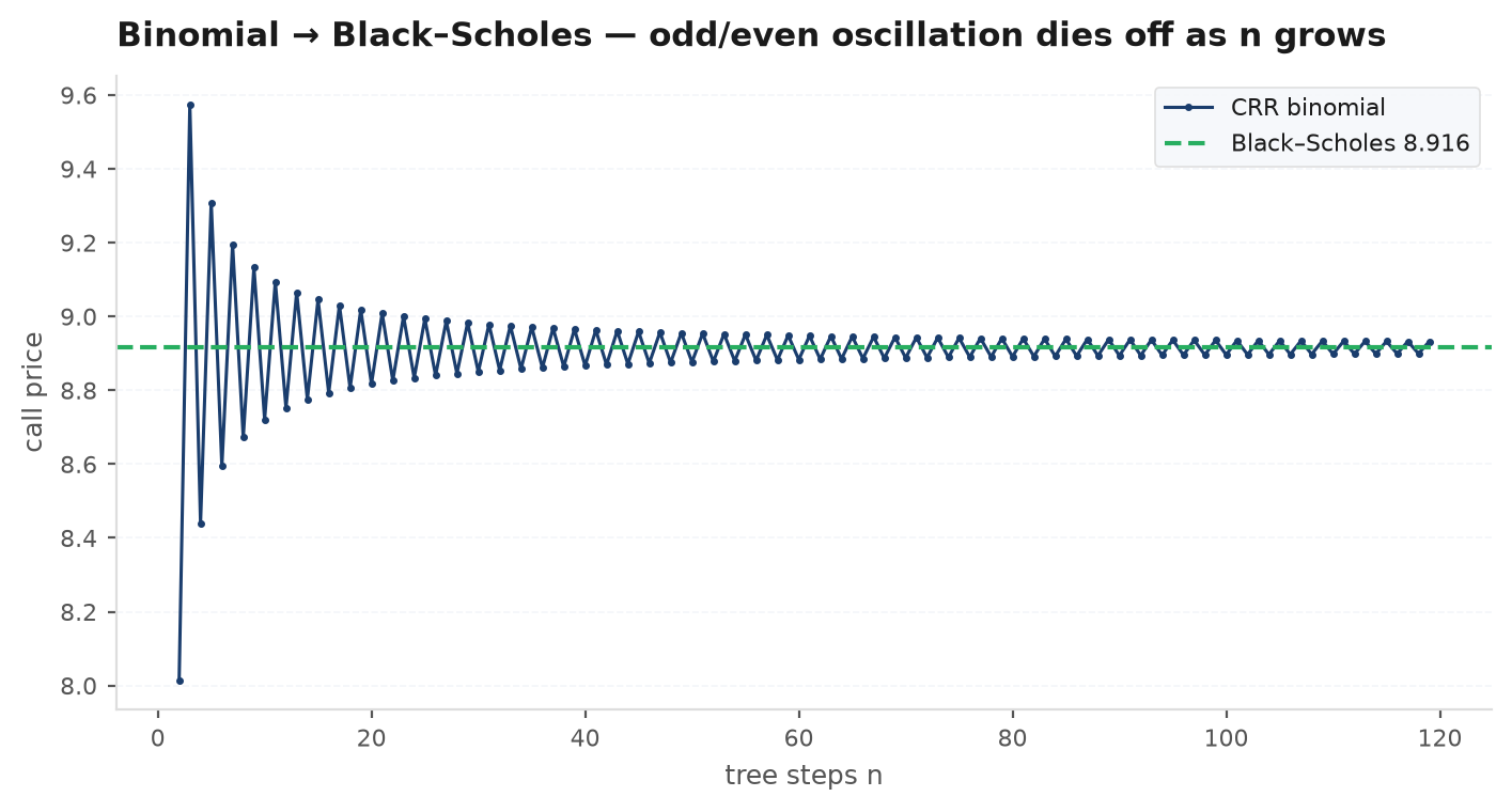
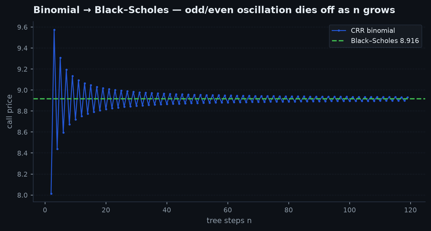
Price by backward induction: at expiry the option is worth its payoff at each terminal node; step backwards, each node’s value is the discounted expectation $e^{- r Δ t} (p V_{up} + (1 - p) V_{down})$ — and for an American option, the maximum of that and immediate exercise. That one extra $max$ is why trees matter: early exercise breaks every closed form, and the tree handles it for free. As $n \to \infty$ the binomial terminal distribution converges (CLT again) to the log-normal of GBM, and the European tree price converges to Black-Scholes with error $O (1/ n)$ — visibly oscillating around the true value as strikes fall between or on node levels.

Binomial tree option price versus number of steps, oscillating around and converging to the Black-Scholes value, with the error envelope shrinking like one over n — CRR tree price vs steps n, against the Black-Scholes closed form (horizontal line). The tree price oscillates — even/odd step counts straddle the strike differently — inside an envelope that shrinks like 1/n. By n = 500 the error is sub-cent; the American premium is then the gap the closed form cannot see.

tree.py

import edgekit as ek

# American put on the house scenario: S=100, K=100, T=1y, r=5%, sigma=20%.
amer = ek.options.binomial_tree(100, 100, 1.0, 0.05, 0.20, n=500, kind="put", american=True)

# Same tree, European exercise — converges to Black-Scholes as n grows.
euro = ek.options.binomial_tree(100, 100, 1.0, 0.05, 0.20, n=500, kind="put", american=False)

amer - euro    # > 0: the early-exercise premium, priced by one extra max()

Monte Carlo, and why variance reduction pays#

Crude Monte Carlo prices by simulating $n$ paths and averaging discounted payoffs $Y_{i}$ . The standard error is $σ_{Y} / n$ — to halve it, quadruple the paths. Variance reduction attacks $σ_{Y}$ instead of $n$ .

Antithetic variates#

Simulate paths in mirrored pairs: for every draw of Gaussian shocks $Z$ , also run $- Z$ , and average the pair’s payoffs $Y ˉ = \frac{1}{2} (Y + Y^{'})$ .

✦Derivation — variance of the pair average

For the average of two identically-distributed estimates with correlation $ρ = Corr (Y, Y^{'})$ :

Var (\frac{Y + Y ^{'}}{2}) = \frac{1}{4} (σ^{2} + σ^{2} + 2 ρ σ^{2}) = \frac{σ ^{2}}{2} (1 + ρ) .

Independent pairs ( $ρ = 0$ ) give $σ^{2} /2$ — exactly what two plain paths give, no gain. But if the payoff is monotone in the shocks (a call is: bigger shocks, bigger payoff), then $Y^{'} = g (- Z)$ is anticorrelated with $Y = g (Z)$ , $ρ < 0$ , and the pair average beats two independent paths — at half the random-number cost, since each pair reuses its draws. When one path lands high, its mirror lands low; the errors cancel by construction. For payoffs that are close to linear in the shocks, $ρ \to - 1$ and the variance nearly vanishes.

Control variates#

Pair each payoff $Y$ with a correlated quantity $X$ whose true mean you know — for options, the terminal price itself: $E [S_{T}] = S_{0} e^{r T}$ under the risk-neutral measure. Then estimate with the corrected average

θ^= Y ˉ - β (X ˉ - E [X]) .

Whatever luck pushed the simulated $X ˉ$ above its known mean also pushed $Y ˉ$ up; subtracting $β$ times the observable error removes the shared luck. Minimising $Var (θ^) = Var (Y) - 2 β Cov (Y, X) + β^{2} Var (X)$ over $β$ gives the optimal coefficient and the payoff:

β^{*} = \frac{Cov ( Y , X )}{Var ( X )}, Var (θ^) = σ_{Y}^{2} (1 - ρ_{X Y}^{2}) .

The same $β$ as an OLS slope, and the same $1 - ρ^{2}$ as a regression’s unexplained variance — this is regression, applied to simulation error. With $ρ = 0.95$ , variance drops $10 \times$ ; at $ρ = 0.99$ , $50 \times$ .

Low-discrepancy sequences#

Random points clump and leave voids — that irregularity is the $1/ n$ . Quasi-Monte Carlo abandons randomness for sequences engineered to fill space evenly. The Halton sequence builds coordinate $j$ by reflecting the integers written in base $p_{j}$ (the $j$ -th prime) about the decimal point: in base 2 the sequence runs $\frac{1}{2}, \frac{1}{4}, \frac{3}{4}, \frac{1}{8}, \frac{5}{8}, \dots$ — each new point landing in the largest remaining gap. Integration error for such sequences obeys the Koksma-Hlawka bound,

error = O (\frac{( lo g n ) ^{d}}{n}) vs O (n^{- 1/2}) for Monte Carlo,

which is nearly $1/ n$ in modest dimension $d$ — a square-root improvement in the exponent, worth orders of magnitude at large $n$ . The $(lo g n)^{d}$ factor is the warning label: as $d$ grows the advantage fades (in practice QMC still wins well past the bound’s pessimism, because payoffs concentrate their variance in a few effective dimensions). Push Halton uniforms through the inverse normal CDF and you have evenly-spaced Gaussians ready for any path simulator from Simulating markets.

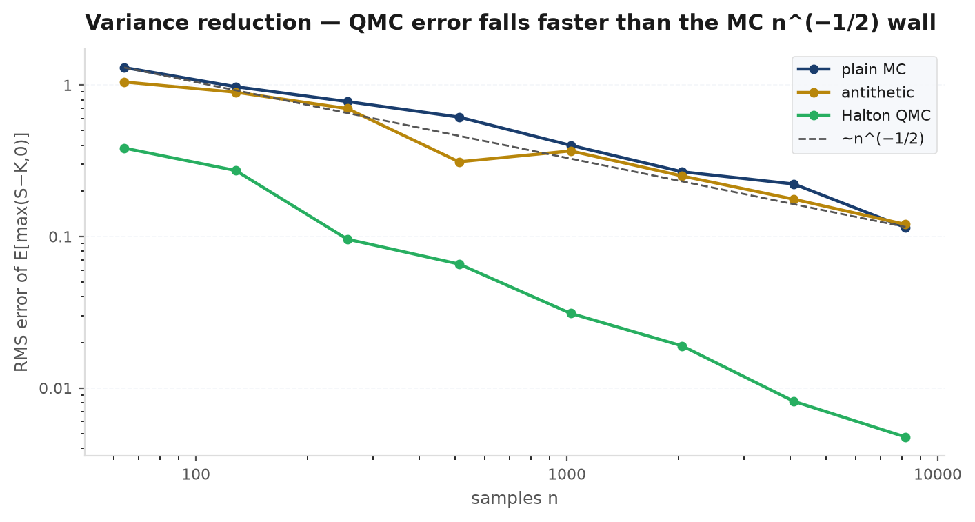
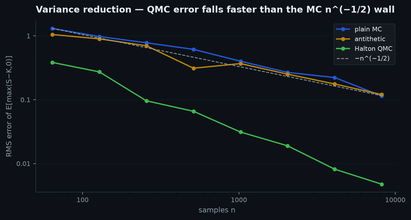
Log-log plot of pricing error versus number of paths for crude Monte Carlo, antithetic variates, control variates, and Halton quasi-Monte Carlo, showing parallel one-half slopes with lower constants and a steeper slope for quasi-Monte Carlo — Error vs n for pricing the same option, log-log. Crude MC falls with slope −1/2; antithetic and control variates run parallel but lower — same rate, smaller constant, with the control variate's drop set by 1−rho². The Halton line falls with slope near −1: a different exchange rate entirely.

✦Scenario — one option, four methods

Price the European call with $S = K = 100$ , $T = 1$ , $r = 5%$ , $σ = 20%$ . Black-Scholes says $C = 10.45$ — the target. A CRR tree is within a cent by $n \approx 200$ steps (error $\sim 1/ n$ ). Crude Monte Carlo with $n = 10, 000$ paths: the discounted payoff has $σ_{Y} \approx 14.7$ , so the standard error is $14.7/ 1 0^{4} \approx 0.15$ — a penny and a half of noise per dollar of option. Antithetic pairing ( $ρ \approx - 0.6$ for this payoff) cuts the variance by $1 + ρ$ , standard error to roughly $0.07$ . A control variate on $S_{T}$ ( $ρ_{X Y} \approx 0.94$ at the money) multiplies variance by $1 - 0.9 4^{2} \approx 0.12$ : standard error $\approx 0.05$ , a $9 \times$ path saving. Halton quasi-normals at the same $n$ land within about a cent. Moral: before buying compute, spend ten lines of code — the tricks stack, and together they buy a $10 - 100 \times$ effective speed-up.

variance_reduction.py

import numpy as np
import edgekit as ek

S0, K, T, r, sigma = 100.0, 100.0, 1.0, 0.05, 0.20
n = 10_000
disc = np.exp(-r * T)

def terminal(z):                       # exact GBM terminal price from N(0,1) draws
    return S0 * np.exp((r - 0.5 * sigma**2) * T + sigma * np.sqrt(T) * z)

# 1) Antithetic: second half of draws is the negation of the first.
z = ek.sim.antithetic(n)[:, 0]
pay = disc * np.maximum(terminal(z) - K, 0.0)
est_anti = pay.mean()

# 2) Control variate: S_T has known risk-neutral mean S0 * e^{rT}.
st = terminal(np.random.default_rng(11).standard_normal(n))
y = disc * np.maximum(st - K, 0.0)
cv = ek.sim.control_variate(y, st, S0 * np.exp(r * T))
cv["estimate"], cv["beta"], cv["var_reduction"]

# 3) Quasi-Monte Carlo: Halton points -> normals -> paths.
zq = ek.sim.quasi_normals(n)[:, 0]      # norm_ppf(halton), evenly spaced draws
est_qmc = (disc * np.maximum(terminal(zq) - K, 0.0)).mean()

Choosing a method#

Method	Error rate	Best for	Breaks down when
Newton root-finding	quadratic (digits double)	implied vol, yields — smooth monotone f	flat vega / bad start; keep a bisection bracket
Simpson quadrature	O(h^4)	1-D expectations with known density	dimension > ~3 (grid explodes)
CRR binomial tree	O(1/n)	American / early-exercise features	path-dependence, many state variables
MC + variance reduction	O(1/sqrt(n)), smaller constant	high dimensions, any payoff	control poorly correlated; payoff non-monotone (antithetic)
Quasi-MC (Halton)	~O((log n)^d / n)	smooth payoffs, moderate d	large d; naive error bars (points are not random)

!Quasi-random points have no standard error

A Halton estimate comes with no honest confidence interval — the points are deterministic, so the usual

σ^/ n

is meaningless (and flattered by the even spacing). Practice randomises the sequence (a random shift or scramble per replication) to recover error bars. And all variance reduction shares one caveat: it sharpens the estimate of the model’s price. If the model is GBM and reality has jumps and fat tails, you now have a beautifully precise wrong answer — the gap that Monte-Carlo methods stress-tests with fatter-tailed generators.

Next: what happens when the object you estimate is an entire matrix — and most of its eigenvalues are noise. Random matrix theory.