Maximum likelihood & method of moments

The previous chapter judged estimators; this one manufactures them. Maximum likelihood is the master recipe: write down the probability of the data as a function of the parameter, and pick the parameter that makes what you saw least surprising. It is invariant, asymptotically normal, and asymptotically efficient — it attains the Cramér–Rao floor in the limit. But it has famous failure modes (the uniform, mixtures), and its humbler cousin, the method of moments, is often the right first move. Mastery means knowing the derivations, the one non-regular case, and the asymptotics.

✦Intuition — likelihood is probability read backwards

A density $f (x; θ)$ answers “given the parameter, how probable is this data?” The likelihood fixes the observed data $x_{1}, \dots, x_{n}$ and reads the same formula as a function of $θ$ : $L (θ) = \prod_{i} f (x_{i}; θ)$ . It is not a probability distribution over $θ$ (that requires a prior — Bayesian inference); it is a relative-plausibility ranking. The MLE $θ^$ is its argmax — in practice the argmax of the log-likelihood $ℓ (θ) = \sum_{i} ln f (x_{i}; θ)$ , because sums beat products and the log changes nothing about the maximiser.

The recipe, and five canonical MLEs#

The regular-case recipe: write $ℓ (θ)$ , set the score $ℓ^{'} (θ) = 0$ , solve, and check the second derivative is negative. The five derivations below cover almost every case you will meet.

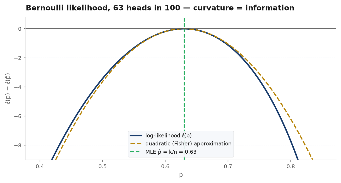
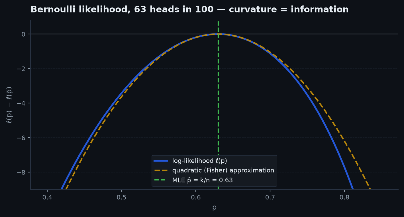
Bernoulli( $p$ ). With $k = \sum x_{i}$ heads, $ℓ (p) = k ln p + (n - k) ln (1 - p)$ ; $ℓ^{'} (p) = k / p - (n - k) / (1 - p) = 0$ gives $p^= k / n$ . Sixty-two heads in 100 tosses: $p^= 0.62$ .

Poisson( $λ$ ). $ℓ (λ) = - nλ + \sum x_{i} ln λ - \sum ln x_{i}!$ , so $ℓ^{'} = - n + \sum x_{i} / λ = 0$ gives $λ^= x ˉ$ — the sample mean of counts.

Exponential( $λ$ ). $ℓ (λ) = n ln λ - λ \sum x_{i}$ , so $λ^= 1/ x ˉ$ . Five order-arrival gaps ${0.3, 0.9, 1.2, 0.4, 0.7}$ seconds: $x ˉ = 0.7$ , $λ^\approx 1.43$ per second.

✦Derivation — normal (μ, σ²), and the biased σ̂²

For $N (μ, σ^{2})$ ,

ℓ (μ, σ^{2}) = - \frac{n}{2} ln (2 π σ^{2}) - \frac{1}{2 σ ^{2}} i \sum (x_{i} - μ)^{2} .

$\partial ℓ / \partial μ = \frac{1}{σ ^{2}} \sum (x_{i} - μ) = 0$ gives $μ^= x ˉ$ regardless of $σ^{2}$ . Substituting and setting $\partial ℓ / \partial σ^{2} = - \frac{n}{2 σ ^{2}} + \frac{1}{2 σ ^{4}} \sum (x_{i} - x ˉ)^{2} = 0$ gives

σ^^{2} = \frac{1}{n} i \sum (x_{i} - x ˉ)^{2} = \frac{n - 1}{n} s^{2} .

The MLE divides by $n$ , so $E [σ^^{2}] = \frac{n - 1}{n} σ^{2}$ : biased low by $σ^{2} / n$ (the proof that $E [s^{2}] = σ^{2}$ is in estimators & sampling). MLE does not promise unbiasedness — it promises asymptotic optimality, and the bias vanishes at rate $1/ n$ .

Log-likelihood surface for a normal model over mu and sigma, peaked at the sample mean and the MLE sigma, with contour lines showing curvature — The normal log-likelihood surface. The MLE is the peak; the curvature at the peak is the observed information, and sharper curvature means a tighter sampling distribution — the geometry behind the I(theta)^-1 asymptotic variance.

Uniform $[0, θ]$ — the non-regular case. The likelihood is not smooth in $θ$ :

L (θ) = θ^{- n} 1 {θ \geq i max x_{i}} .

No derivative is ever zero — $θ^{- n}$ is strictly decreasing — so the maximum sits on the boundary of the allowed region: $θ^= max_{i} x_{i}$ . Setting derivatives to zero here is the classic trap; the support depends on the parameter, the regularity conditions fail, and (as shown in the previous chapter) the estimator converges at rate $1/ n$ rather than $1/ n$ , with $n (θ - θ^)$ converging to an exponential — not a normal — distribution.

Invariance — the free lunch#

Theorem (invariance). If $θ^$ is the MLE of $θ$ , then for any function $g$ , $g (θ^)$ is the MLE of $η = g (θ)$ .

✦Proof — invariance of the MLE

If $g$ is one-to-one, the likelihood of $η$ is $L^{g} (η) = L (g^{- 1} (η))$ ; since $L$ is maximised at $θ^$ , $L^{g}$ is maximised exactly at $η = g (θ^)$ . For general $g$ , define the induced (profile) likelihood $L^{g} (η) = sup_{θ : g (θ) = η} L (θ)$ . For every $η$ , $L^{g} (η) \leq L (θ^)$ , and the value $η = g (θ^)$ attains that ceiling because $θ^$ belongs to its preimage. Hence $g (θ^)$ maximises $L^{g}$ . Use it: the MLE of an exponential tail probability $P (X > 1) = e^{- λ}$ is just $e^{- λ^} = e^{- 1.43} \approx 0.24$ from the worked data above — no new optimisation. Note the contrast with unbiasedness, which is destroyed by nonlinear $g$ (Jensen); invariance is the property unbiasedness wishes it had.

Asymptotics — why MLE wins in the limit#

Under regularity (smooth density, support free of $θ$ , information $I (θ)$ finite and positive), the MLE from an iid sample satisfies

n (θ^- θ_{0}) d N (0, I (θ_{0})^{- 1}),

so the MLE is consistent, asymptotically normal, and asymptotically efficient: its limiting variance is the Cramér–Rao floor $1/ (n I (θ_{0}))$ derived in estimators & sampling.

✦Proof sketch — expand the score

The MLE solves $ℓ^{'} (θ^) = 0$ . Taylor-expand the score around the truth $θ_{0}$ :

0 = ℓ^{'} (θ^) \approx ℓ^{'} (θ_{0}) + ℓ^{''} (θ_{0}) (θ^- θ_{0}) ⟹ n (θ^- θ_{0}) \approx \frac{ℓ ^{'} ( θ _{0} ) / n}{- ℓ ^{''} ( θ _{0} ) / n} .

The numerator is a scaled sum of iid score terms with mean 0 and variance $I (θ_{0})$ , so by the CLT it converges to $N (0, I (θ_{0}))$ . The denominator is an average of iid terms with mean $I (θ_{0})$ , so by the LLN it converges to $I (θ_{0})$ . Slutsky’s theorem combines them: $N (0, I) / I = N (0, I^{- 1})$ . Consistency itself needs a separate uniform-convergence argument (the average log-likelihood converges to its expectation, which is maximised at $θ_{0}$ by Jensen applied to $ln (f_{θ} / f_{θ_{0}})$ — the Kullback–Leibler inequality).

Observed vs expected information. In practice $I (θ_{0})$ is unknown; two plug-ins compete. The expected information evaluates the formula $n I (θ^)$ ; the observed information uses the actual curvature of your sample, $J (θ^) = - ℓ^{''} (θ^)$ . Both are consistent; Efron and Hinkley’s classic argument favours the observed one — it conditions on how much information this sample happened to carry. Standard errors are then $se (θ^) = J (θ^)^{- 1/2}$ . Worked number: for the exponential, $I (λ) = 1/ λ^{2}$ , so with $n = 5, λ^= 1.43$ : $se \approx λ^/ n = 0.64$ — five observations pin down almost nothing, which is exactly what the width says.

Method of moments#

The method of moments (MoM) predates likelihood: equate as many sample moments to model moments as there are parameters, and solve. It requires no optimisation, works when the likelihood is ugly, and by the LLN plus the continuous-mapping theorem is consistent whenever the moment map is invertible and continuous.

Gamma(shape $α$ , rate $β$ ): mean $α / β$ , variance $α / β^{2}$ . Matching $x ˉ$ and $s^{2}$ gives $α^= x ˉ^{2} / s^{2}$ , $β^= x ˉ / s^{2}$ . Data with $x ˉ = 2, s^{2} = 8$ : $α^= 0.5$ , $β^= 0.25$ . The gamma MLE has no closed form (it involves the digamma function) — MoM hands you the answer, or the starting point for the numeric MLE.
Student- $t$ degrees of freedom: a standardised $t_{ν}$ has variance $ν / (ν - 2)$ for $ν > 2$ . Matching the sample variance $s^{2}$ gives $ν^= 2 s^{2} / (s^{2} - 1)$ : daily returns standardised to variance $3$ imply $ν^= 3$ — the fat-tail regime where the fourth moment is already infinite (see the distribution zoo).

	Maximum likelihood	Method of moments
Efficiency	Asymptotically efficient (attains CR bound)	Generally inefficient
Requirements	Full density, regularity, optimisation	Just moments and the LLN
Robustness to misspecification	Can be badly wrong if the density is wrong	Only needs the moment structure to be right
Typical role	Final estimate + standard errors	Closed forms, starting values, quick checks

When likelihood breaks#

The regularity conditions are not decoration; each failure mode is a classic follow-up question.

Parameter-dependent support (Uniform $[0, θ]$ ): no score equation, boundary maximum, $1/ n$ rate, non-normal limit — everything above.
Unbounded likelihood(Gaussian mixtures): put one component’s mean on a data point and let its $σ \to 0$ — the likelihood diverges to infinity at a useless “solution.” Honest fixes: constrain the variance ratio, penalise, or go Bayesian. In practice EM finds a good local maximum and everyone quietly ignores the global degeneracy.
Nuisance parameters: maximise the ones you do not care about away — the profile likelihood $L_{p} (ψ) = sup_{η} L (ψ, η)$ behaves like a likelihood for $ψ$ in regular problems and is how the invariance proof above generalises.

→Quant lens — every fitted model on a desk is an MLE

GARCH volatility models, jump-diffusions, and regime-switching models are all fit by maximising a likelihood — usually a quasi-likelihood: a Gaussian $ℓ$ maximised over returns that are not Gaussian. QMLE still delivers consistent parameter estimates for the conditional-variance dynamics (the moment structure is right even when the density is wrong — the MoM lesson in disguise), but the standard errors must be corrected. The practical workflow mirrors this chapter: MoM or sample statistics for starting values, numerical maximisation of $ℓ$ , observed information for error bars, and suspicion at any likelihood surface as flat as five data points make it. See the applied fit in ARIMA & GARCH and the jump models in jumps & stochastic vol.

Simulation — asymptotic normality, and the non-regular exception#

Two headline claims, verified: the exponential MLE is asymptotically $N (λ, λ^{2} / n)$ , and the uniform MLE is biased by exactly $- θ / (n + 1)$ with its $1/ n$ correction.

mle_asymptotics.py

import numpy as np

rng = np.random.default_rng(11)
reps, n = 100_000, 50

# Regular case: exponential(lambda = 2), MLE = 1/xbar
lam = 2.0
lam_hat = 1.0 / rng.exponential(1 / lam, size=(reps, n)).mean(axis=1)
print(f"E[lam_hat] = {lam_hat.mean():.4f}  (true 2; small-sample bias lam/(n-1) = {lam/(n-1):.4f})")
print(f"sd[lam_hat] = {lam_hat.std():.4f}  vs asymptotic lam/sqrt(n) = {lam/np.sqrt(n):.4f}")

# Non-regular case: Uniform(0, 1), MLE = max, bias -theta/(n+1)
mx = rng.uniform(0, 1, size=(reps, n)).max(axis=1)
print(f"E[max] = {mx.mean():.4f}  vs n/(n+1) = {n/(n+1):.4f}")
print(f"E[(n+1)/n * max] = {((n + 1) / n * mx).mean():.4f}  (bias-corrected)")

Note the regular case’s residual bias $λ / (n - 1)$ : since $\sum X_{i} \sim Gamma (n, λ)$ , $E [1/ X ˉ] = nλ / (n - 1)$ exactly — MLEs are typically biased at order $1/ n$ , and it does not matter asymptotically.

Practice problems#

→Problem 1 — Uniform MLE vs method of moments

For Uniform $[0, θ]$ , compare the MLE $θ^_{M L} = max X_{i}$ with the MoM estimator, and rank them.

Solution. The mean is $θ /2$ , so MoM gives $θ^_{M M} = 2 X ˉ$ : unbiased with variance $4 \cdot \frac{θ ^{2} /12}{n} = \frac{θ ^{2}}{3 n}$ . The MLE has $E [θ^_{M L}] = \frac{n}{n + 1} θ$ (bias $- θ / (n + 1)$ ) and $MSE = \frac{2 θ ^{2}}{( n + 1 ) ( n + 2 )}$ ; the corrected $\frac{n + 1}{n} max X_{i}$ is unbiased with variance $\frac{θ ^{2}}{n ( n + 2 )}$ . Ranking: corrected MLE $(1/ n^{2})$ crushes MoM $(1/ n)$ — for $n = 100$ , roughly a 30-fold smaller standard error. Also note $θ^_{M M}$ can be smaller than an observed data point — an estimate the data already contradicts, which is the memorable knock against it.

→Problem 2 — MLE under censoring

Lifetimes are Exponential( $λ$ ). You observe $d$ exact failure times $t_{1}, \dots, t_{d}$ , and $m$ units still alive at time $c$ (right-censored). Find the MLE.

Solution. A failure contributes density $λ e^{- λ t_{i}}$ ; a censored unit contributes survival probability $e^{- λ c}$ . So $ℓ (λ) = d ln λ - λ (\sum_{i} t_{i} + m c)$ , and

λ^= \frac{d}{\sum _{i} t _{i} + m c} = \frac{events}{total time at risk} .

Numeric: 3 defaults at years $1, 2, 4$ and 2 names surviving 5 years: $λ^= 3/ (7 + 10) \approx 0.176$ per year. The estimator is the occurrence/exposure rate — the form actuaries, credit-risk desks, and reliability engineers all use, and a neat example of the likelihood handling partial information that MoM cannot digest.

→Problem 3 — Moments for a mixture

Returns are drawn from an equal mixture of $N (μ, 1)$ and $N (- μ, 1)$ (a crude two-regime model). Estimate $μ$ by moments. Why not first moments?

Solution. By symmetry $E [X] = 0$ for every $μ$ — the first moment is blind. Go to the second: conditioning on the component, $E [X^{2}] = μ^{2} + 1$ . So match $m_{2} = \frac{1}{n} \sum x_{i}^{2}$ :

μ^= m_{2} - 1, (set μ^= 0 if m_{2} < 1) .

The truncation at zero is the tell that the parameter sits near a boundary where regular asymptotics warp. The mixture MLE has no closed form (and the unbounded-likelihood pathology if variances are also free) — this is the standard example of MoM succeeding where naive likelihood maximisation is treacherous.

→Problem 4 — Why use a biased σ̂²?

The normal MLE $σ^^{2}$ divides by $n$ and is biased. Why does anyone prefer it to $s^{2}$ ?

Solution. Three reasons, in ascending depth. (1) MSE: $MSE (σ^^{2}) = \frac{2 n - 1}{n ^{2}} σ^{4} < \frac{2}{n - 1} σ^{4} = MSE (s^{2})$ for all $n$ — the bias buys more variance than it costs (and $1/ (n + 1)$ beats both; see estimators & sampling). (2) Invariance: $σ^= σ^^{2}$ is the MLE of $σ$ , while no divisor makes both $s^{2}$ and $s$ unbiased simultaneously (Jensen), so chasing unbiasedness is chasing a moving target. (3) Asymptotics: the difference is $O (1/ n)$ , inside the $O (1/ n)$ sampling noise — the choice is invisible exactly when the estimate is trustworthy.

→Problem 5 — A one-line MLE

For the density $f (x; θ) = θ x^{θ - 1}$ on $(0, 1)$ with $θ > 0$ , find the MLE and its asymptotic variance.

Solution. $ℓ (θ) = n ln θ + (θ - 1) \sum_{i} ln x_{i}$ , so $ℓ^{'} = n / θ + \sum ln x_{i} = 0$ gives $θ^= - n / \sum_{i} ln x_{i}$ . The trick worth saying aloud: $Y = - ln X \sim Exponential (θ)$ , so this is the exponential MLE in disguise, and immediately $I (θ) = 1/ θ^{2}$ , giving asymptotic variance $θ^{2} / n$ — transformation first, computation second.

Next: estimators in hand, decide between hypotheses — type I and II errors, p-values and their misreadings, power, and the confidence-interval duality. Hypothesis tests & confidence intervals.