Regression & Gauss–Markov

Ordinary least squares is the single most-used statistical tool in finance — every beta, every alpha, every factor loading is a regression coefficient. This chapter builds OLS from two directions (calculus and geometry), states the Gauss–Markov assumptions with full precision and proves the BLUE property, derives the two great failure formulas — omitted-variable bias and measurement-error attenuation — and finishes with regression to the mean, the statistical illusion most often mistaken for skill.

✦Intuition — a slope is a covariance in disguise

Everything in this chapter flows from one identity: the fitted slope of $y$ on $x$ is $β^= Cov (x, y) / Var (x)$ — how much $y$ co-moves with $x$ , per unit of $x$ ’s own movement. Once you see that, the pathologies become mechanical: leave out a variable correlated with $x$ and its covariance leaks into the numerator (omitted-variable bias); add noise to $x$ and the denominator inflates while the numerator does not (attenuation). Diagnosing a regression is an audit of one fraction.

OLS view one — calculus and the normal equations#

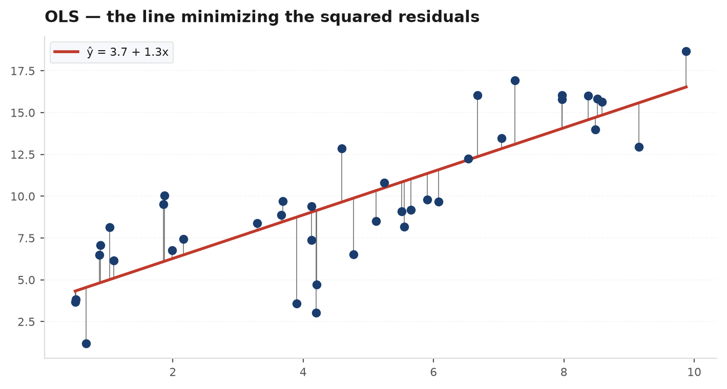
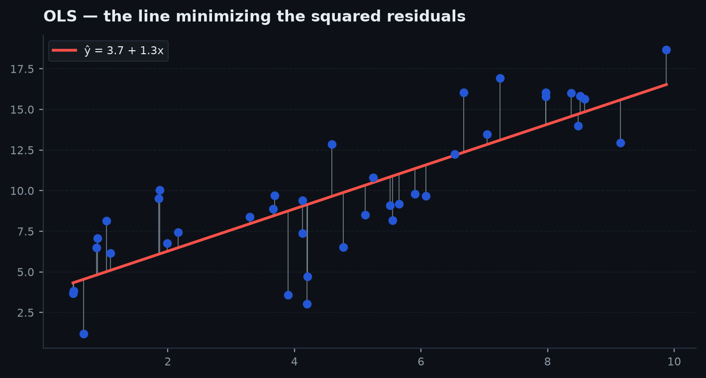
Data $(x_{i}, y_{i})$ , model $y_{i} = α + β x_{i} + ε_{i}$ . OLS picks the line minimising the residual sum of squares $S (α, β) = \sum_{i} (y_{i} - α - β x_{i})^{2}$ . Setting both partial derivatives to zero gives the normal equations:

\frac{\partial S}{\partial α} = - 2 i \sum (y_{i} - α - β x_{i}) = 0, \frac{\partial S}{\partial β} = - 2 i \sum x_{i} (y_{i} - α - β x_{i}) = 0.

The first says residuals sum to zero (the line passes through $(x ˉ, y ˉ)$ ); substituting it into the second and solving:

β^= \frac{\sum _{i} ( x _{i} - x ˉ ) ( y _{i} - y ˉ )}{\sum _{i} ( x _{i} - x ˉ ) ^{2}} = \frac{Cov ( x , y )}{Var ( x )} = ρ^\frac{s _{y}}{s _{x}}, α^= y ˉ - β^x ˉ .

In matrix form with design matrix $X$ (a column of ones plus regressors), minimise $∥ y - X β ∥^{2}$ ; the gradient $- 2 X^{⊤} (y - X β) = 0$ gives $X^{⊤} X β^= X^{⊤} y$ , hence $β^= (X^{⊤} X)^{- 1} X^{⊤} y$ whenever $X^{⊤} X$ is invertible.

✦Worked example — a regression by hand

Data: $x = (1, 2, 3, 4, 5)$ , $y = (2, 2, 4, 4, 6)$ . Then $x ˉ = 3$ , $y ˉ = 3.6$ , $S_{xx} = 4 + 1 + 0 + 1 + 4 = 10$ , and $S_{x y} = (- 2) (- 1.6) + (- 1) (- 1.6) + 0 + (1) (0.4) + (2) (2.4) = 10$ . So

β^= 10/10 = 1.0, α^= 3.6 - 3 = 0.6.

Residuals $(0.4, - 0.6, 0.4, - 0.6, 0.4)$ sum to zero as required; $RSS = 1.2$ , $TSS = 11.2$ , so $R^{2} = 1 - 1.2/11.2 \approx 0.89$ . The error variance estimate is $s^{2} = RSS / (n - 2) = 0.4$ , giving $se (β^) = s^{2} / S_{xx} = 0.2$ and $t = 1.0/0.2 = 5.0$ on 3 degrees of freedom ( $p \approx 0.015$ ) — a slope this clean in five points is already strong evidence.

OLS view two — geometry and projection#

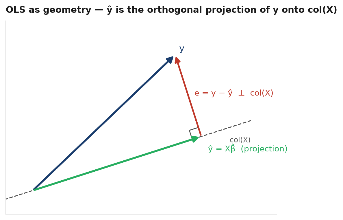
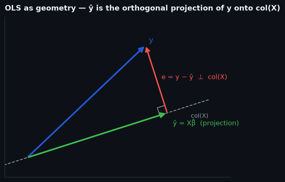
The fitted values are $y^= X β^= X (X^{⊤} X)^{- 1} X^{⊤} y = H y$ , where $H$ is the hat matrix. Check its two defining properties: $H^{⊤} = H$ and $H^{2} = X (X^{⊤} X)^{- 1} X^{⊤} X (X^{⊤} X)^{- 1} X^{⊤} = H$ — a symmetric idempotent matrix, i.e. an orthogonal projection. OLS projects the data vector $y$ onto the column space of $X$ ; the residual vector $e = (I - H) y$ is what is left, and it is orthogonal to every regressor by construction:

X^{⊤} e = X^{⊤} (y - X β^) = X^{⊤} y - X^{⊤} X β^= 0 (the normal equations, re-read) .

Pythagoras then gives the variance decomposition $∥ y - y ˉ 1 ∥^{2} = ∥ y^- y ˉ 1 ∥^{2} + ∥ e ∥^{2}$ (TSS = ESS + RSS), and $R^{2}$ is the squared cosine of the angle between the centred $y$ and its projection. Every regression fact has a picture: adding a regressor enlarges the subspace, so RSS can only fall — which is exactly why raw $R^{2}$ is gameable.

Vector diagram of the data vector projected orthogonally onto the plane spanned by the regressors, with the residual perpendicular to the plane — OLS as orthogonal projection: y is dropped perpendicularly onto the span of the regressors; the fitted value is the shadow, the residual the perpendicular. Residuals orthogonal to regressors is not an assumption — it is the definition of the estimator.

The Gauss–Markov theorem#

When is OLS not just a line but the best one? The assumptions must be stated exactly — the hardest questions live in the gap between the folklore version and the real one. For the model $y = X β + ε$ :

GM1 — linearity: the data are generated by $y = X β + ε$ for some true $β$ (linear in parameters; $X$ may contain squares, logs, dummies).
GM2 — strict exogeneity: $E [ε ∣ X] = 0$ . The errors have mean zero given every observation of every regressor. This is the assumption OVB, simultaneity, and measurement error all violate — the load-bearing one.
GM3 — no perfect collinearity: $rank (X) = k$ , so $(X^{⊤} X)^{- 1}$ exists.
GM4 — spherical errors: $Var (ε ∣ X) = σ^{2} I$ — homoskedastic (equal variance) and uncorrelated across observations.

Note what is absent: no normality, no i.i.d. regressors, nothing about causality. Theorem (Gauss–Markov). Under GM1–GM4, the OLS estimator $β^$ is BLUE: among all estimators that are linear in $y$ and unbiased, it has the smallest variance (in the positive semi-definite ordering — smallest variance for every linear combination of coefficients).

✦Proof sketch — BLUE

Any linear estimator is $β ~ = C y$ . Write $C = (X^{⊤} X)^{- 1} X^{⊤} + D$ . Unbiasedness for all $β$ requires $E [β ~] = C X β = β$ , i.e. $C X = I$ , which forces $D X = 0$ . Then, using GM4,

Var (β ~) = σ^{2} C C^{⊤} = σ^{2} [(X^{⊤} X)^{- 1} + D D^{⊤}],

because the cross terms contain $D X = 0$ . Since $D D^{⊤}$ is positive semi-definite, $Var (β ~) ⪰ σ^{2} (X^{⊤} X)^{- 1} = Var (β^)$ , with equality iff $D = 0$ . QED. Every deviation from OLS that stays linear and unbiased adds variance — the theorem is an accounting identity once you see the decomposition. But note its limits: drop unbiased and shrinkage estimators (ridge, Bayesian posteriors from last chapter) can beat OLS on MSE; drop GM4 and GLS is better.

Adding normality of errors upgrades algebra to exact distributions: $β^\sim N (β, σ^{2} (X^{⊤} X)^{- 1})$ , $(n - k) s^{2} / σ^{2} \sim χ_{n - k}^{2}$ independent of $β^$ , so each coefficient’s $t_{j} = (β^_{j} - β_{j}^{0}) / se (β^_{j}) \sim t_{n - k}$ — the same machinery as hypothesis testing. Joint restrictions use the F statistic $F = \frac{( RSS _{r} - RSS _{u} ) / q}{RSS _{u} / ( n - k )}$ . For fit, $R^{2} = 1 - RSS / TSS$ never decreases when regressors are added; adjusted $R ˉ^{2} = 1 - (1 - R^{2}) \frac{n - 1}{n - k}$ charges a small rent per regressor — but the honest referee is out-of-sample performance, not any in-sample statistic (overfitting detection).

Scatter of points with the fitted least-squares line and vertical residual segments from each point to the line — The fitted line minimises the sum of squared vertical distances. Note the asymmetry baked into the objective: x is treated as given, y as noisy — which is why regressing y on x and x on y give different lines (Problem 1).

Omitted-variable bias — derived#

Suppose the truth involves two regressors, $y = β_{1} x_{1} + β_{2} x_{2} + ε$ (variables centred, GM2 holding in the long model), but you run the short regression of $y$ on $x_{1}$ alone.

✦Derivation — the OVB formula

The short slope is the covariance ratio; substitute the true model into it:

b_{1} = \frac{Cov ( x _{1} , y )}{Var ( x _{1} )} = \frac{Cov ( x _{1} , β _{1} x _{1} + β _{2} x _{2} + ε )}{Var ( x _{1} )} = β_{1} + β_{2} δ_{21} \frac{Cov ( x _{1} , x _{2} )}{Var ( x _{1} )} .

So short = long + effect of omitted × regression of omitted on included: $bias = β_{2} δ_{21}$ , where $δ_{21}$ is the slope you would get regressing $x_{2}$ on $x_{1}$ . The bias vanishes only if the omitted variable is irrelevant ( $β_{2} = 0$ ) or uncorrelated with the included one ( $δ_{21} = 0$ ). The sign is the product of the two signs — which is why you can reason out the direction of a bias without any numbers.

	Cov(x₁, x₂) > 0	Cov(x₁, x₂) < 0
β₂ > 0 (omitted helps y)	upward bias	downward bias
β₂ < 0 (omitted hurts y)	downward bias	upward bias

Measurement error — attenuation, derived#

Now suppose the model is clean, $y = β x + ε$ , but you observe $x$ only through noise: $x^{*} = x + u$ , with $u$ independent of $x$ and $ε$ , variance $σ_{u}^{2}$ . Regressing $y$ on $x^{*}$ :

b \to \frac{Cov ( x ^{*} , y )}{Var ( x ^{*} )} = \frac{Cov ( x + u , β x + ε )}{σ _{x}^{2} + σ _{u}^{2}} = β λ \in (0, 1) \frac{σ _{x}^{2}}{σ _{x}^{2} + σ _{u}^{2}} .

The numerator keeps only $β σ_{x}^{2}$ (noise is uncorrelated with everything), while the denominator inflates by $σ_{u}^{2}$ . The slope is multiplied by the reliability ratio $λ$ — always attenuated toward zero, never inflated. Signal-to-noise 1:1 halves your measured beta. In quant work the regressor is almost always estimated (a signal, a factor exposure, a past beta), so raw cross-sectional slopes on estimated quantities are systematically too flat — the root of beta shrinkage (Problem 5).

Both failure formulas are two-line simulations — verify them:

ovb_attenuation_check.py

import numpy as np

rng = np.random.default_rng(11)
n, beta1, beta2 = 200_000, 1.0, 0.5

# omitted-variable bias: Cov(x1,x2)=0.6 -> short slope = 1 + 0.5*0.6 = 1.30
x1 = rng.standard_normal(n)
x2 = 0.6 * x1 + 0.8 * rng.standard_normal(n)
y = beta1 * x1 + beta2 * x2 + rng.standard_normal(n)
b_short = np.cov(x1, y)[0, 1] / x1.var()
print(f"short slope {b_short:.3f}   OVB formula {beta1 + beta2 * 0.6:.3f}")

# attenuation: sigma_u = 0.5 -> lambda = 1/(1+0.25) = 0.80
x_obs = x1 + 0.5 * rng.standard_normal(n)
y2 = beta1 * x1 + rng.standard_normal(n)
b_att = np.cov(x_obs, y2)[0, 1] / x_obs.var()
print(f"noisy slope {b_att:.3f}   attenuation formula {beta1 / 1.25:.3f}")

When the error assumptions fail#

Multicollinearity (GM3 stressed). With correlated regressors the variance of $β^_{j}$ is $σ^{2} / (n Var (x_{j}) (1 - R_{j}^{2}))$ , where $R_{j}^{2}$ comes from regressing $x_{j}$ on the other regressors. The variance inflation factor $VIF_{j} = 1/ (1 - R_{j}^{2})$ quantifies the damage: $R_{j}^{2} = 0.9$ means VIF 10, standard errors $\times 10 \approx 3.2$ . Estimates stay unbiased but individual coefficients become unstable while the joint fit is fine — highly collinear factor exposures produce exactly this signature.

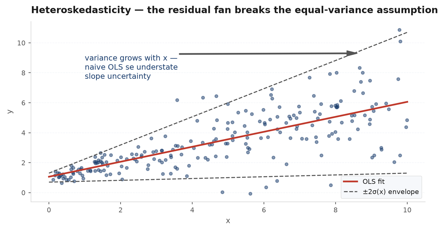
Heteroskedasticity (GM4a broken). If $Var (ε_{i} ∣ X) = σ_{i}^{2}$ varies, OLS remains unbiased and consistent, but it is no longer BLUE and — the practical disaster — the textbook standard errors are simply wrong, usually too small where high-variance points align with extreme $x$ . The fix is not to re-estimate the slope but the uncertainty: White’s robust (sandwich) estimator $(X^{⊤} X)^{- 1} (\sum_{i} e_{i}^{2} x_{i} x_{i}^{⊤}) (X^{⊤} X)^{- 1}$ lets each observation report its own squared residual.

Autocorrelation (GM4b broken). With serially correlated errors — routine in finance: overlapping returns, persistent volatility — effective sample size shrinks by the $(1 + 2 \sum_{k} ρ_{k})$ factor derived in LLN & CLT, and naive standard errors overstate precision. Newey–West / HACstandard errors extend the sandwich with cross-products at nearby lags, downweighted linearly out to a chosen bandwidth. edgekit’s factor utilities apply these by default (factors API); see also time-series statistics.

Scatter with a fan-shaped spread of residuals widening with x, fitted line overlaid, illustrating heteroskedastic errors — Heteroskedasticity: the residual spread fans out with x. The fitted slope is still unbiased, but textbook standard errors — which assume one sigma for all points — misreport uncertainty; robust (White) errors reweight by each point's own squared residual.

Regression to the mean#

The name “regression” comes from Galton’s discovery, and the phenomenon is a theorem about the bivariate normal derived in joint distributions: if $(X, Y)$ are bivariate normal with correlation $ρ$ , then

E [Y ∣ X = x] = μ_{Y} + ρ \frac{σ _{Y}}{σ _{X}} (x - μ_{X}) ⟹ E [Z_{Y} ∣ Z_{X} = z] = ρ z .

In standardised units, the predicted outcome is the observed one shrunk by $ρ$ . Whenever $∣ ρ ∣ < 1$ , extreme observations are followed, on average, by less extreme ones — with no causal mechanism whatsoever. Model performance as skill + luck: the skill component repeats, the luck redraws, so the year-2 expectation of a year-1 outlier is pulled toward the mean by exactly the fraction of variance that was luck. The sophomore slump, the “curse” of magazine covers, and most hot-hand fund narratives are this equation wearing costumes. Numeric: fund returns with year-to-year correlation 0.3; a fund that just printed a $+ 2 σ$ year has expected next year $0.3 \times 2 = + 0.6 σ$ — still good, but the naive extrapolation is off by 70% of its excess.

!Regression is association, not causation

Gauss–Markov says nothing about why x and y co-move. GM2 fails silently under simultaneity (price and volume cause each other), selection (you only observe surviving funds — survivorship), and confounding (OVB above). A regression coefficient is a conditional-mean slope in the sampled population; promoting it to “if I change x, y will respond by beta” requires causal assumptions no amount of fit statistics can supply. Every quant blow-up story features a regression read causally that was merely associational.

→Quant lens — alpha, beta, and the factor regression

The canonical desk regression is $r_{t}^{strat} = α + β r_{t}^{mkt} + ε_{t}$ : $β$ measures hedgeable market exposure, $α$ the residual edge, and the t-stat on $α$ is the strategy’s real report card — a strategy can have a glowing Sharpe that is nothing but $β \times$ a bull market. Everything in this chapter bites at once: returns are heteroskedastic and autocorrelated (use HAC errors), factor exposures are estimated with noise (attenuation), omitting a factor the strategy loads on inflates $α$ (OVB — the “alpha” of a small-cap strategy regressed only on the market is mostly the omitted size factor). Multi-factor extensions and edgekit’s implementation live in regression & factor models.

Practice problems#

→Problem 1 — regress y on x, then x on y

The slope of y on x is $b_{y x}$ ; of x on y is $b_{x y}$ . What is $b_{y x} b_{x y}$ ? Why isn’t $b_{x y} = 1/ b_{y x}$ ?

Solution. $b_{y x} = ρ σ_{y} / σ_{x}$ and $b_{x y} = ρ σ_{x} / σ_{y}$ , so the product is $ρ^{2} = R^{2}$ . They are mutual inverses only when $∣ ρ ∣ = 1$ . The reason: each regression minimises errors in its own vertical direction, shrinking its slope toward zero by a factor $ρ$ relative to the SD line (slope $σ_{y} / σ_{x}$ ). In standardised units both slopes equal $ρ < 1$ — both predictions regress to the mean, in opposite directions. This is the algebraic heart of the previous section.

→Problem 2 — duplicate every observation

You copy your dataset so every point appears twice, then rerun OLS. What happens to $β^$ , the standard errors, and the t-stats? What real situation does this parody?

Solution. The normal equations scale by 2 on both sides, so $β^$ , the residuals, $R^{2}$ , and $s^{2}$ are all unchanged. But the reported variance $s^{2} (X^{⊤} X)^{- 1}$ halves (as $X^{⊤} X$ doubles), so standard errors shrink by $2$ and t-stats inflate by $2$ — with zero new information. The software believed GM4’s “uncorrelated errors” while you fed it perfectly correlated pairs. That is precisely what autocorrelated returns or overlapping windows do covertly: observations that are partial copies of each other. Effective n, not nominal n, sets precision — the fix is HAC errors or non-overlapping sampling.

→Problem 3 — sign the omitted-variable bias

You regress stock returns on a value signal, omitting momentum. Momentum predicts returns positively, and value and momentum scores are negatively correlated. Is your value coefficient biased up or down?

Solution. By the OVB formula, bias $= β_{mom} \times δ$ where $δ$ is the slope of momentum on value. Here $β_{mom} > 0$ and $δ < 0$ , so the bias is negative: the short regression understatesvalue’s effect, because every high-value name drags in a momentum headwind that gets billed to the value signal. Controlling for momentum would raise the value coefficient. The two-sign product rule answers any variant in one breath — then add the caveat that if the “omitted” variable is a collider or a consequence of the included one, controlling for it introduces bias instead (Problem 4).

→Problem 4 — when should you add a control?

Adding a control variable: always safer? When does it help, and when does it actively hurt?

Solution. Add a control when it is a confounder — it affects $y$ and correlates with your regressor of interest: that removes OVB by moving its covariance out of the error term (restoring GM2). It hurts when: (i) it is a consequence of the regressor (post-treatment) — controlling for it absorbs part of the very effect you are measuring; (ii) it is a collider(both x and y affect it) — conditioning opens a spurious path (Berkson’s paradox, next chapter); (iii) it is nearly collinear with x — no bias, but VIF blows up your standard errors. The one-line answer: controls are causal decisions, not statistical hygiene — you need a story about the arrows, not just a bigger $R^{2}$ .

→Problem 5 — why shrink estimated betas?

Market betas estimated on 60 months are used to predict next-period betas. The cross-sectional regression of realised on estimated betas has slope well below 1. Why, and what is the fix?

Solution. An estimated beta is the true beta plus estimation noise: $β^_{i} = β_{i} + u_{i}$ . Predicting anything from $β^$ is a regression on a noisy regressor, so the slope is attenuated by the reliability $λ = σ_{β}^{2} / (σ_{β}^{2} + σ_{u}^{2})$ — mechanical measurement-error attenuation, not mean-reversion in true betas (though that adds too). The fix is to shrink each estimate toward the cross-sectional mean: $β_{i}^{adj} = λ β^_{i} + (1 - λ) \times 1$ — Vasicek’s adjustment, which is exactly the precision-weighted normal–normal posterior of the previous chapterwith the cross-section as prior (Blume’s 0.67/0.33 rule is the fixed-weight folk version). One phenomenon, three names: attenuation, shrinkage, empirical Bayes.

Next:one regression is inference; fifty regressions until one works is a different sport with different rules — and most published “alpha” loses to them. Multiple testing & paradoxes.