Multiple testing & paradoxes

A single hypothesis test controls its error rate. A searchover many hypotheses does not — and almost everything a quant does is a search. This chapter builds the machinery for testing many things at once (FWER, Bonferroni, Holm, FDR, Benjamini–Hochberg), derives the $2 ln N$ law for the best of $N$ random strategies, and then tours the paradoxes — Simpson’s, Berkson’s, regression to the mean — that make honest-looking data lie.

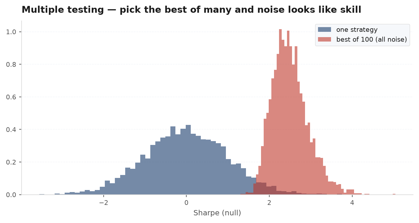
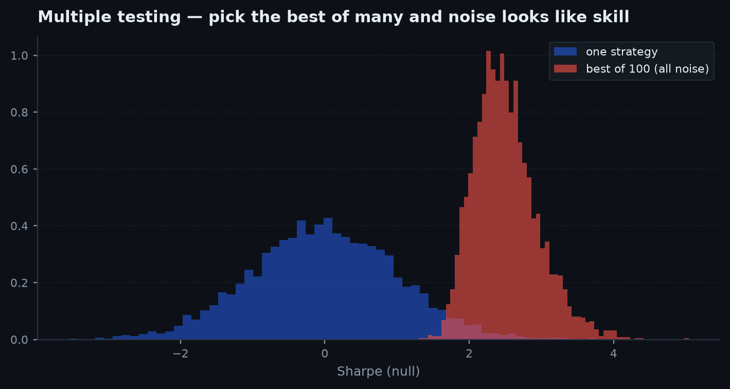
✦Intuition — the lottery you accidentally run

One fair coin flipped 100 times almost never shows 60 heads. But hand a coin to a thousand people and someone will — with near certainty. Multiple testing is the discipline of remembering how many coins you handed out. Every parameter grid, every universe scan, every discarded variant of a backtest is another coin, and the best result you keep is the maximum of many draws, not a typical draw. The mathematics of maxima is brutal: the expected best of $N$ pure-noise strategies grows like $2 ln N$ standard errors — slowly, but relentlessly. Everything in this chapter is a defence against being fooled by your own search.

The multiplicity problem and FWER#

Suppose you run $m$ hypothesis tests, each at level $α$ . Under the global null (all $m$ nulls true), each test has probability $α$ of a false rejection. The family-wise error rate is the probability of making at least one false rejection:

FWER = P (V \geq 1), V = # {false rejections} .

If the tests are independent, $FWER = 1 - (1 - α)^{m}$ . With $m = 20$ and $α = 0.05$ :

1 - 0.9 5^{20} = 1 - 0.358 = 0.642.

A 64% chance of at least one “significant” discovery from pure noise — and the expected number of false positives is $m α = 1$ exactly, by linearity of expectation over indicator variables (see Random variables & moments). One spurious winner per twenty tries is not bad luck; it is the arithmetic default.

Probability of at least one false positive rising quickly toward one as the number of independent tests grows — FWER as a function of the number of tests at alpha = 0.05. By 14 tests you are more likely than not to have at least one false positive; by 60 it is near certainty. A parameter sweep is a family of tests whether you call it one or not.

Bonferroni and Holm#

The oldest fix is Bonferroni: test each hypothesis at level $α / m$ .

✦Proof — Bonferroni controls FWER, via the union bound

Let $A_{i}$ be the event that true null $i$ is falsely rejected, so $P (A_{i}) \leq α / m$ . The union bound (Boole’s inequality, proved in Inequalities & tail bounds) gives

FWER = P (i \in true nulls ⋃ A_{i}) \leq i \sum P (A_{i}) \leq m_{0} \cdot \frac{α}{m} \leq α,

where $m_{0} \leq m$ is the number of true nulls. No independence assumption is used anywhere — Bonferroni is valid under arbitrary dependence between the tests, which is why it survives in finance where every test shares the same underlying prices. The price of that robustness is conservatism: with correlated tests the effective number of independent looks is smaller than $m$ , and Bonferroni over-corrects.

Holm’s step-down procedure dominates Bonferroni at no cost. Sort the p-values $p_{(1)} \leq \dots \leq p_{(m)}$ and compare $p_{(k)}$ against $α / (m - k + 1)$ , rejecting sequentially until the first failure, then stopping. The smallest p-value still faces $α / m$ , but each subsequent one faces a looser bar because a rejection removes one hypothesis from the family. Holm controls FWER under arbitrary dependence too (same union bound applied to the remaining nulls at each step) and never rejects fewer hypotheses than Bonferroni — there is no reason to ever prefer plain Bonferroni.

False discovery rate and Benjamini–Hochberg#

FWER is the right target when a single false positive is catastrophic. But in a screen of 10,000 signals you do not need zero false discoveries — you need the proportion of your discoveries that are false to be small. That is the false discovery rate:

FDR = E [\frac{V}{max ( R , 1 )}],

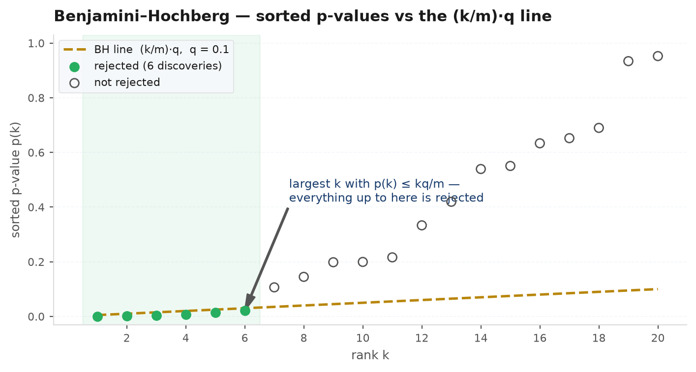
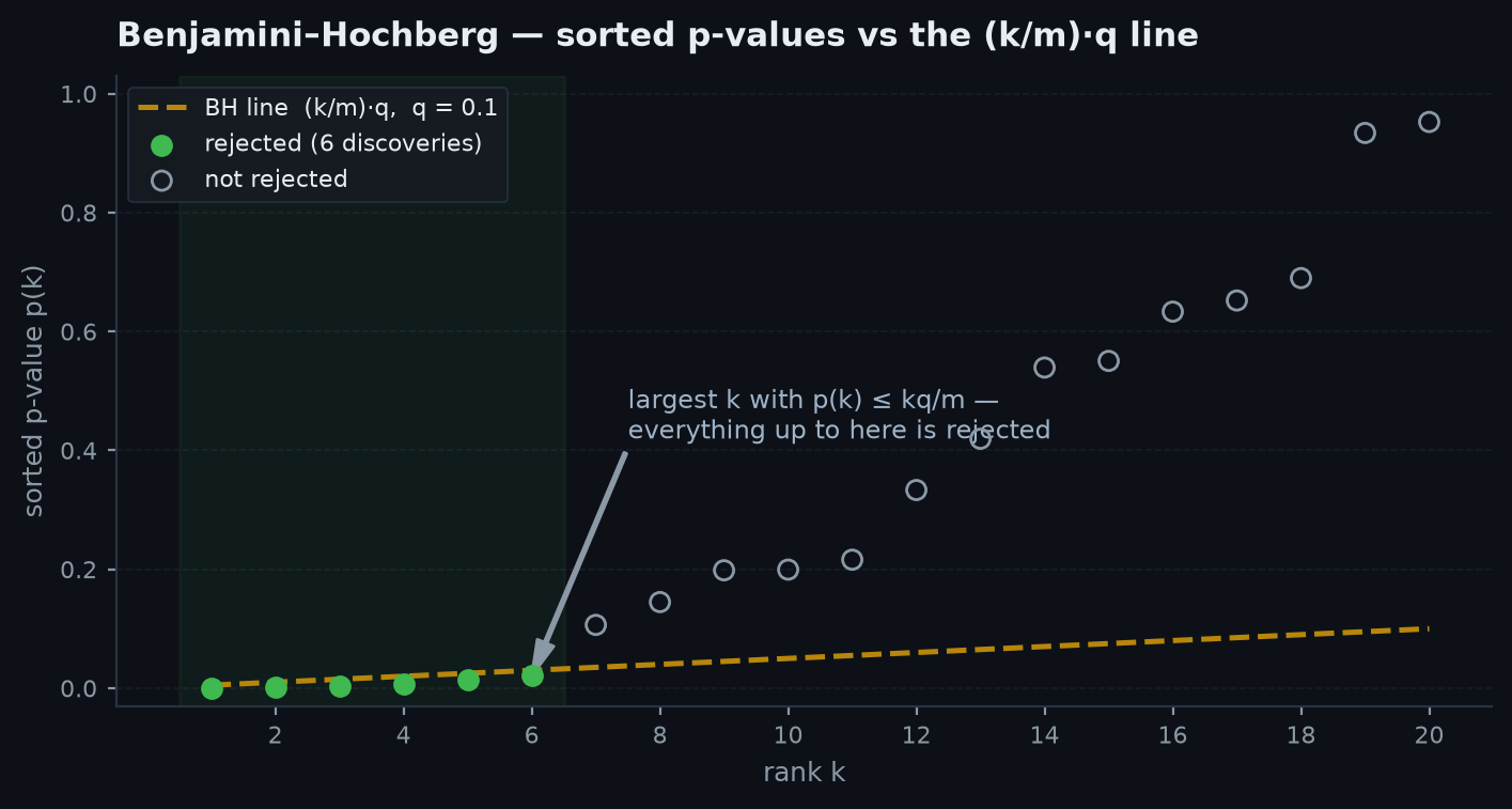
where $R$ is the total number of rejections. The Benjamini–Hochberg procedure at level $q$ : sort the p-values, find the largest $k$ with

p_{(k)} \leq \frac{k}{m} q,

and reject hypotheses $1, \dots, k$ . Under independent (or positively dependent) p-values, BH guarantees $FDR \leq \frac{m _{0}}{m} q \leq q$ .

✦Proof sketch — why the BH line works

The intuition: if you reject everything with $p \leq t$ , the true nulls contribute about $m_{0} t$ false discoveries (null p-values are Uniform(0,1), by the probability integral transform proved in Order statistics), while the observed count of discoveries is $R (t)$ . The estimated FDR at threshold $t$ is therefore $FDR (t) \approx m t / R (t)$ . Setting $t = p_{(k)}$ , where $R = k$ , the condition $m p_{(k)} / k \leq q$ is exactly the BH rule: choose the most generous threshold whose estimated false-discovery proportion is still below $q$ . The formal proof (Benjamini & Hochberg 1995) makes this exact with a clever martingale argument, showing the expectation is bounded by $m_{0} q / m$ .

Worked example (by hand). Five signals produce p-values $0.005, 0.011, 0.020, 0.040, 0.130$ ; take $q = 0.05$ . The BH thresholds $k q / m$ are $0.01, 0.02, 0.03, 0.04, 0.05$ . Compare in order: 0.005 ≤ 0.01 ✓, 0.011 ≤ 0.02 ✓, 0.020 ≤ 0.03 ✓, 0.040 ≤ 0.04 ✓, 0.130 ≤ 0.05 ✗. The largest passing index is $k = 4$ , so BH rejects the first four. Bonferroni at the same level tests each against $0.05/5 = 0.01$ and rejects only one. That is the trade: BH buys power by tolerating a controlled fraction of false discoveries instead of forbidding them.

Sorted p-values plotted against rank with the rising Benjamini-Hochberg line, rejections below the largest crossing highlighted — Benjamini-Hochberg by picture: sorted p-values against the line kq/m. Everything up to the last point under the line is rejected — including points that individually sit above the line, which is what makes BH a step-up procedure rather than a per-test threshold.

Data snooping: the expected maximum Sharpe of N random strategies#

Now the quant version, and the headline derivation of the chapter. You backtest $N$ strategies that are all pure noise over $T$ observations. Each estimated Sharpe ratio is approximately Gaussian around zero (CLT; see LLN & the CLT) with standard error $σ_{S R} \approx 1/ T$ in per-period units. What does the best one look like?

✦Derivation — E[max] of N standard normals is about sqrt(2 ln N)

Let $Z_{1}, \dots, Z_{N}$ be iid standard normal and $M_{N} = max_{i} Z_{i}$ . Upper bound. The Gaussian tail obeys $P (Z > x) \leq e^{- x^{2} /2}$ for $x \geq 0$ (Chernoff bound). By the union bound,

P (M_{N} > x) \leq N P (Z > x) \leq N e^{- x^{2} /2},

which drops below any $ε$ once $x^{2} /2 > ln (N / ε)$ , i.e. just above $2 ln N$ . Lower bound. For $x = (1 - δ) 2 ln N$ , the tail satisfies $P (Z > x) ≳ e^{- x^{2} /2} / x = N^{- (1 - δ)^{2}} / x$ , so the expected number of exceedances $N P (Z > x) \to \infty$ . By independence,

P (M_{N} \leq x) = (1 - P (Z > x))^{N} \leq e^{- N P (Z > x)} \to 0.

Squeezed from both sides, $M_{N} / 2 ln N \to 1$ in probability, and indeed $E [M_{N}] = 2 ln N (1 + o (1))$ . Scaling by the Sharpe standard error, the expected best in-sample Sharpe of $N$ noise strategies is

E [i max S R_{i}] \approx σ_{S R} 2 ln N .

The growth is only logarithmic — but $2 ln 100 \approx 3.0$ and $2 ln 1000 \approx 3.7$ standard errors. With one year of daily data the annualised Sharpe standard error is about 1, so the best of a thousand random strategies shows a Sharpe near 3.7. This is the mathematical core of the deflated Sharpe ratio and of overfitting detection: any reported Sharpe must be judged against the number of trials that produced it.

Worked numbers. One year of daily data, $T = 252$ . The annualised Sharpe estimate under the null has standard error $252 / 252 = 1.0$ . Searching $N = 50$ parameter combinations: $2 ln 50 = 7.82 \approx 2.80$ . Your grid search is expected to hand you a Sharpe-2.8 strategy from pure noise. A backtest that reports Sharpe 2.5 after trying 50 variants has, on this evidence alone, found nothing.

max_sharpe_of_noise.py

import numpy as np

rng = np.random.default_rng(11)
N, T = 1000, 252                       # 1000 noise strategies, 1 year of daily returns
rets = rng.normal(0.0, 0.01, size=(N, T))   # zero-edge daily returns

sr = np.sqrt(252) * rets.mean(axis=1) / rets.std(axis=1, ddof=1)
print(f"best in-sample Sharpe : {sr.max():.2f}")
print(f"sqrt(2 ln N) theory   : {np.sqrt(2*np.log(N)):.2f}")
print(f"share with SR > 2     : {(sr > 2).mean():.3f}")
# best in-sample Sharpe : ~3.7   -- matches sqrt(2 ln 1000) = 3.72
# a full ~2% of pure-noise strategies clear the 'Sharpe 2' bar

→Quant lens — why out-of-sample decay is the norm, not bad luck

The selected maximum is biased upward by construction: conditional on being the best of

N

, a strategy’s in-sample Sharpe equals its (possibly zero) true skill plus a maximum-of-noise term of order

2 ln N / T

. Out of sample the noise term resets to mean zero, so performance drops by exactly the selection bonus on average — even if the strategy is genuinely good. This is regression to the mean wearing a trading costume, and it is why Why backtests lie treats the number of trials as a first-class input, and why the honest fixes are out-of-sample data the search never touched, Bonferroni/BH-style haircuts on t-statistics, or deflated Sharpe ratios.

The garden of forking paths#

Explicit grids are the easy case — at least $N$ is countable. The insidious version is the garden of forking paths (Gelman’s phrase): choices made after seeing the data that would have been made differently had the data looked different. Each fork is a silent test. The taxonomy every quant should recognise in their own work:

Parameter snooping: tuning lookbacks, thresholds, exits until the equity curve looks right — the explicit grid.
Universe selection:the strategy “works on tech stocks” because 11 sectors were tried and one passed.
Period selection:starting the backtest in 2009 (conveniently after the crash) or excluding “unrepresentative” regimes.
Metric shopping: reporting Sharpe when Sortino is bad, hit rate when Sharpe is bad, CAGR when both are bad.
Outlier surgery:removing the one trade that “was a data error” — after noticing it was the worst trade.
Stopping rules: ending the research project the week the result is significant (the sequential-peeking problem from Hypothesis tests).

Publication and survivorship bias are the same phenomenon at the level of the ecosystem: journals publish the significant results, fund databases contain the funds that survived. A fund graveyard is a filter on the maximum — the industry-wide average track record you observe is conditioned on survival, which is conditioned on past returns. Roughly half of all funds in major databases at inception have disappeared within a decade; averaging the survivors overstates realised returns by percentage points per year. When you evaluate a universe of managers or published anomalies, you are always looking at order statistics, never at typical draws.

Simpson’s paradox#

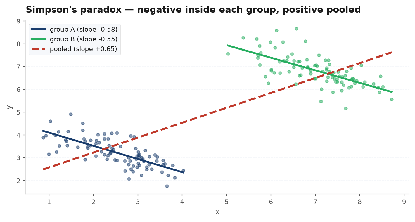
Multiple testing corrupts inference by selection. The paradoxes corrupt it by aggregation. Simpson’s paradox: a relationship that holds in every subgroup can reverse when the groups are pooled. A trading example with concrete numbers — two execution algos, split by market regime:

	Calm days: fills ok / total	Volatile days: fills ok / total	Overall
Algo A	81/87 (93%)	192/263 (73%)	273/350 (78%)
Algo B	234/270 (87%)	55/80 (69%)	289/350 (83%)

Algo A is better on calm days (93% vs 87%) and better on volatile days (73% vs 69%) — yet worse overall (78% vs 83%). No arithmetic error: A was routed mostly to volatile days (263 of 350), where everyone does badly, while B enjoyed mostly calm days. The pooled comparison is confounded by the regime mix. Formally, with regime $R$ and algo $T$ ,

P (ok ∣ T) = r \sum P (ok ∣ T, R = r) P (R = r ∣ T),

and the weights $P (R = r ∣ T)$ differ across algos — the law of total probability with different mixing weights can reverse any inequality.

Two subgroup trends both sloping one way while the pooled trend slopes the opposite way — Simpson's paradox: within each subgroup the relationship points one way; pooling flips it because the groups have different sizes and baselines. The pooled slope answers a different question than the subgroup slopes.

!When to aggregate — the causal answer

There is no purely statistical rule; it depends on the causal structure. If the grouping variable (regime) is a confounder — it influences both which algo is used and the outcome — you must condition on it: the stratified comparison is the honest one, and here A really is the better algo. If instead the grouping variable is a consequence of the treatment (a mediator — e.g. the algo itself causes volatile-looking fills), conditioning on it throws away the effect you care about, and the pooled number is the honest one. Same table, opposite conclusions — the data alone cannot tell you which. Ask where the arrows point before choosing the slice.

Berkson, base rates, and regression to the mean#

Berkson’s paradox is conditioning-on-a-collider: selecting on a common effect of two independent causes makes them negatively correlated in the selected sample. Numeric example: suppose surviving your first year as a fund requires either genuine skill (probability 0.2, independent) or lucky timing (probability 0.3). Among all funds, skill and luck are independent. Among survivors, $P (luck ∣ skill) = 0.3$ but $P (luck ∣ no skill, survived) = 1$ — the unskilled survivors must have been lucky. Skill and luck are now negatively associated, which is why, in any filtered universe (listed funds, published papers, live strategies), good properties appear to trade off against each other even when they are independent in the population.

Base-rate neglect, from Bayes’ theorem, compounds all of this: a “95%-significant” signal is not 95% likely to be real. If only 1 in 100 candidate signals has a true edge, then among signals passing a 5% test with power 0.8, the posterior probability of a real edge is

P (edge ∣ pass) = \frac{0.8 \times 0.01}{0.8 \times 0.01 + 0.05 \times 0.99} = \frac{0.008}{0.0575} \approx 0.14.

Six in seven “discoveries” are false at these base rates — the FDR made personal. Regression to the meancloses the loop: if performance = skill + noise, the top decile of this year’s managers is selected partly on noise, so next year they fall back toward the mean by a factor of the correlation $ρ$ between periods (derived with the bivariate normal in Regression & Gauss–Markov: $E [Z_{2} ∣ Z_{1} = z] = ρ z$ ). “Hot hands cool” needs no story about complacency — it is what selection on a noisy signal does, mechanically.

Practice problems#

→Problem 1 — Twenty strategies, one hits p < 0.05

You test 20 independent strategies against a no-edge null; exactly one comes back with $p = 0.04$ . Is it an edge?

Solution. Under the global null the number of false positives is Binomial(20, 0.05): the expected count is $20 \times 0.05 = 1$ , and $P (at least one) = 1 - 0.9 5^{20} \approx 0.64$ . Observing exactly one marginal p-value is therefore the most typical possible outcome of pure noise — it is evidence of nothing. The slick follow-up: to claim significance you should Bonferroni-correct, requiring $p < 0.05/20 = 0.0025$ ; equivalently the adjusted p-value is $min (20 \times 0.04, 1) = 0.80$ . The finding is fully consistent with zero true edges.

→Problem 2 — Benjamini–Hochberg by hand

Apply BH at $q = 0.10$ to p-values $0.008, 0.028, 0.041, 0.062, 0.400$ . Which are rejected? How does Bonferroni at $α = 0.10$ compare?

Solution. Thresholds $k q / m = k \times 0.02$ : $0.02, 0.04, 0.06, 0.08, 0.10$ . Checks: 0.008 ≤ 0.02 ✓, 0.028 ≤ 0.04 ✓, 0.041 ≤ 0.06 ✓, 0.062 ≤ 0.08 ✓, 0.400 ≤ 0.10 ✗. Largest passing index is $k = 4$ : reject the first four — note the step-up subtlety that 0.041 and 0.062 are rejected even though each alone exceeds some smaller thresholds only matters via the largest k. Bonferroni tests against $0.10/5 = 0.02$ and rejects only the first. BH discovers four signals while promising merely that on average ≤ 10% of discoveries are false; Bonferroni protects against any false discovery and pays for it in power.

→Problem 3 — Simpson reversal, constructed live

A firm’s new model beats the old one in both large-cap and small-cap universes but loses overall. Construct numbers showing this, and say which comparison matters.

Solution.The recipe: make the strata have very different base rates, then give each model a different mix. New model — large-cap 45/50 (90%), small-cap 45/150 (30%), overall 90/200 = 45%. Old model — large-cap 130/150 (87%), small-cap 14/50 (28%), overall 144/200 = 72%. The new model wins each stratum (90% > 87%, 30% > 28%) yet loses overall (45% < 72%) purely because it was deployed mostly in the hard small-cap universe while the old one lived in easy large caps. The stratified comparison is the right one if universe assignment is a confounder (models were routed differently); the causal question — who chose where each model runs, and why — decides, not the arithmetic. The tool to internalise is the mixing identity: pooled rate = Σ (stratum rate × stratum weight), and different weights can reverse any within-stratum ordering.

→Problem 4 — Expected best of N coin-flippers

1,000 analysts each flip a fair coin 10 times; the firm promotes anyone with 10 heads. How many “perfect forecasters” do you expect, and what is the chance there is at least one?

Solution. Per analyst, $P (10 heads) = 2^{- 10} = 1/1024$ . By linearity, expected count $= 1000/1024 \approx 0.98$ — about one. By independence, $P (\geq 1) = 1 - (1 - 1/1024)^{1000} \approx 1 - e^{- 0.977} \approx 0.62$ . So the firm will, more often than not, find someone with a flawless record containing zero information. The general lesson is the $2 ln N$ law in miniature: the best of a large field of noise looks extraordinary, and its expected future performance is exactly the base rate — 50/50 on the next flip.

→Problem 5 — Quantify the selection bonus

A researcher tried $N = 200$ strategy variants on $T = 504$ days (two years) and presents the best, with annualised Sharpe 2.1. Estimate the in-sample Sharpe you would expect from pure noise, and the haircut to apply.

Solution. The annualised Sharpe standard error over two years is roughly $1/ 2 \approx 0.71$ (per-year units: $σ_{S R} \approx 252/ T = 0.5$ ). Expected max of 200 noise draws: $0.71 \times 2 ln 200 = 0.71 \times 3.26 \approx 2.3$ . The presented Sharpe of 2.1 is below the expected best of pure noise given the search size — the correct posterior is that there is no demonstrated edge at all. This is the deflated-Sharpe logic: benchmark the reported maximum against $σ_{S R} 2 ln N$ , not against zero. Expect out-of-sample decay of the full selection bonus even when some skill exists.

→Problem 6 — Why does the top fund underperform next year?

Annual fund returns are $R = S + ε$ with persistent skill $S \sim N (0, 1)$ and fresh noise $ε \sim N (0, 3)$ each year. A fund posts this year’s $R_{1} = 4$ (in the same units). Predict next year.

Solution. Year-over-year correlation: $ρ = Cov (R_{1}, R_{2}) / Var (R) = 1/ (1 + 3) = 0.25$ (only skill persists). By the bivariate-normal conditional mean, $E [R_{2} ∣ R_{1} = 4] = ρ \times 4 = 1$ . Equivalently via Bayes: the posterior mean of skill is $\frac{1}{1 + 3} \times 4 = 1$ (precision weighting, as in Bayesian inference), and next year’s expectation is that posterior skill. The fund is expected to give back three quarters of its outperformance — no story about mean-reverting markets required, just selection on a noisy signal. In a cross-section, the best fund of many is even more noise-loaded than a random 4-sigma fund, so its expected decay is larger still.

Next: the honest way to put error bars on anything — including the selection-biased statistics this chapter warned about — is to resample the data itself. Bootstrap & resampling.