Hypothesis tests & confidence intervals

Testing is the machinery for deciding whether an observed effect — a coin’s excess heads, a strategy’s positive mean return — is signal or noise. This chapter builds the Neyman–Pearson framework properly: what a p-value is (and the catalogue of things it is not), the z and t machinery, the chi-square and F families, the exact duality between confidence intervals and tests, power and sample-size arithmetic, and why peeking at your data inflates false positives. Every corner of quantitative work touches this material, and every backtest silently runs it.

✦Intuition — a test is an asymmetric bet against a null

You never prove anything with data. You pick a boring default (the null: the coin is fair, the strategy has no edge), work out what data it would typically generate, and check whether what you saw is too extreme to sit comfortably in that picture. The asymmetry is deliberate: the null gets the benefit of the doubt, and you control precisely how often you falsely reject it (the level $α$ ). What you do not control by default is how often you miss a real effect — that is power, and it is where most backtests quietly fail.

The Neyman–Pearson framework#

A test has four ingredients: a null hypothesis $H_{0}$ , an alternative $H_{1}$ , a test statistic $T (X)$ whose distribution under $H_{0}$ you know, and a rejection region $R$ . Two errors are possible, and they are not symmetric:

	Reject H₀	Fail to reject H₀
H₀ true	Type I error (prob. α)	Correct (prob. 1 − α)
H₁ true	Correct — power (1 − β)	Type II error (prob. β)

The size (significance level) is $α = P (T \in R ∣ H_{0})$ ; the power against a specific alternative is $1 - β = P (T \in R ∣ H_{1})$ . Fixing $α$ and maximising power is the Neyman–Pearson program, and for simple hypotheses there is a complete answer.

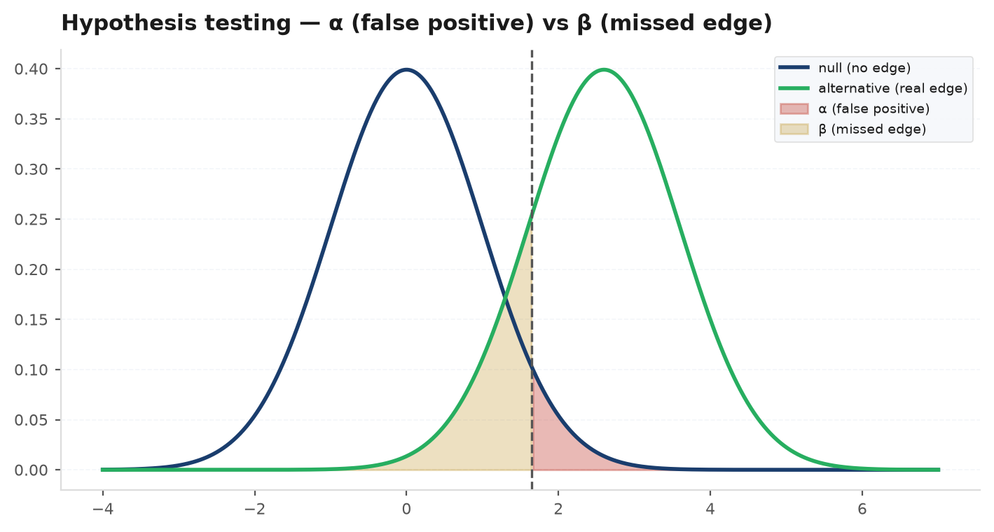
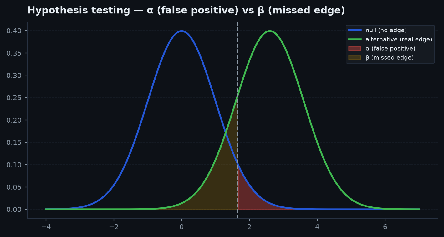
Two overlapping sampling distributions under the null and alternative, with the rejection region shaded in the null's tail and the overlap showing type II error — The geometry of a test: the null's sampling distribution with its alpha-tail shaded (type I error), overlapped by the alternative's distribution. The part of the alternative that falls outside the rejection region is beta — the missed detections. Moving the threshold trades one error for the other; only more data shrinks both.

Neyman–Pearson lemma. For testing a simple null $H_{0} : θ = θ_{0}$ against a simple alternative $H_{1} : θ = θ_{1}$ , the most powerful level- $α$ test rejects exactly when the likelihood ratio is large:

Λ (x) = \frac{L ( θ _{1} ; x )}{L ( θ _{0} ; x )} > k, k chosen so that P_{θ_{0}} (Λ (X) > k) = α .

✦Proof sketch — Neyman–Pearson lemma

Let $φ (x) \in {0, 1}$ be the likelihood-ratio test and $φ^{'} (x)$ any competitor with size at most $α$ . Pointwise, $(φ (x) - φ^{'} (x)) (L_{1} (x) - k L_{0} (x)) \geq 0$ : where $L_{1} > k L_{0}$ the LRT sets $φ = 1 \geq φ^{'}$ , and where $L_{1} < k L_{0}$ it sets $φ = 0 \leq φ^{'}$ — both factors always share a sign. Integrating over $x$ :

(power (φ) - power (φ^{'})) \geq k (α_{φ} - α_{φ^{'}}) \geq 0.

So no test of the same size has more power. The economic intuition: you have an $α$ -budget of null probability to spend on rejections; spend it where each unit of null probability buys the most alternative probability — highest likelihood ratio first, exactly a knapsack argument. This is why likelihood ratios keep reappearing (in the MLE chapter and in Bayes factors next chapter).

The p-value, precisely#

The p-value is the probability, computed assuming the null is true, of obtaining a test statistic at least as extreme as the one observed:

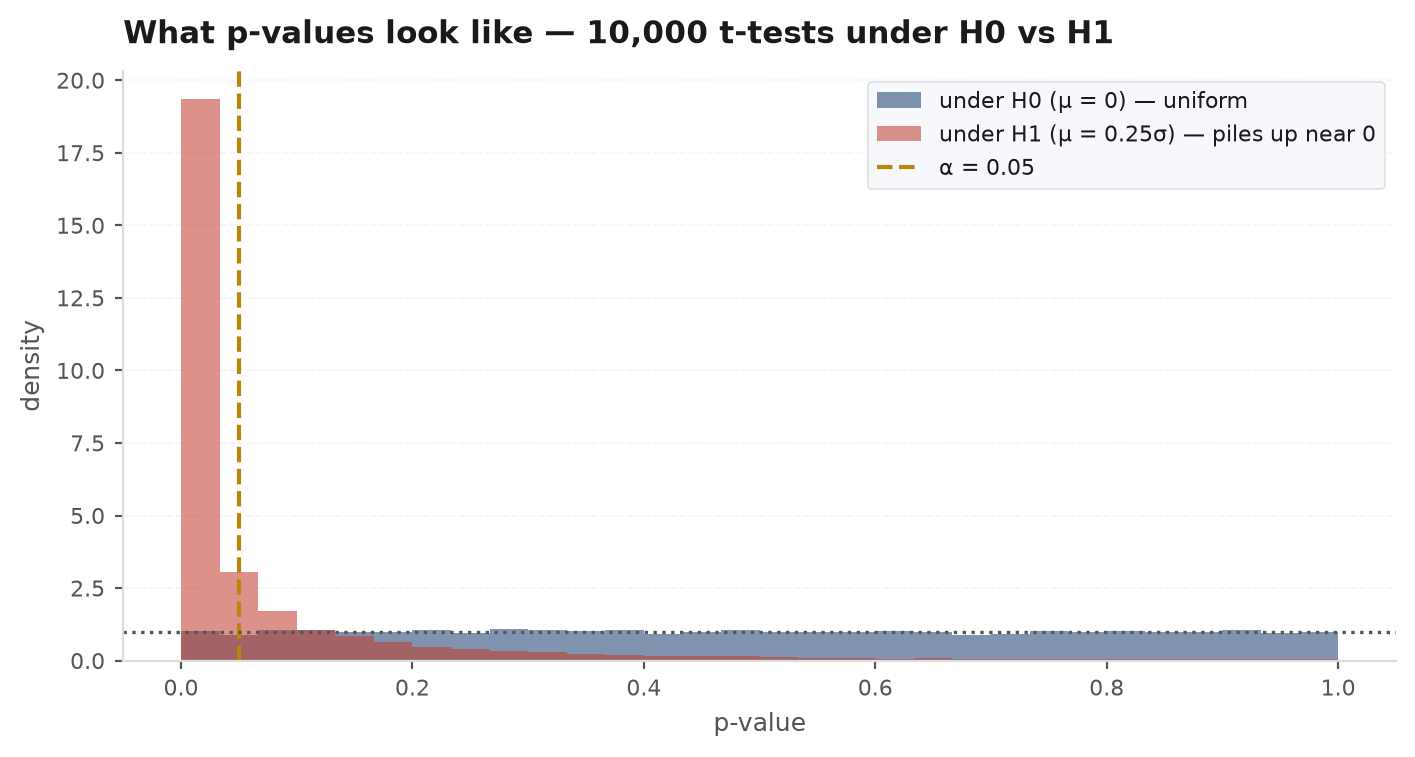
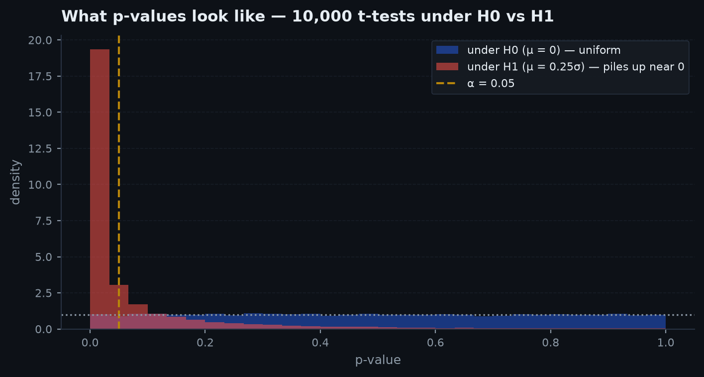
p = P (T \geq t_{obs} ∣ H_{0}) (one-sided; two-sided doubles or uses ∣ T ∣) .

It is a statement about the data given the hypothesis, never about the hypothesis given the data. A key structural fact: if $T$ is continuous with null CDF $F$ , then under $H_{0}$ the p-value $p = 1 - F (T)$ is uniform on [0, 1]. This follows from the probability integral transform proved in order statistics: $F (T) \sim U (0, 1)$ , hence $P (p \leq u) = P (F (T) \geq 1 - u) = u$ . Under the null, p-values carry no information — every value is equally likely, and rejecting when $p \leq α$ gives type I error exactly $α$ . Under an alternative the distribution piles up near zero — that pile-up is power.

Histogram of p-values under the null showing a flat uniform distribution, next to a histogram under a true effect showing p-values piled up near zero — P-values under the null are exactly Uniform(0,1) — the flat histogram. Under a true effect they concentrate near zero; the fraction below alpha is the test's power. A histogram of many p-values that is flat tells you your alternatives are (collectively) not there.

Because the p-value is the most misused number in applied statistics, it pays to probe the failure modes directly. The catalogue:

Claim about p = 0.03	Verdict	Why it fails
“There is a 3% chance the null is true”	False	p conditions on H₀ being true; P(H₀ \| data) needs a prior — that is Bayes, next chapter.
“Only a 3% chance the result is due to chance”	False	Under H₀ the result is 100% due to chance; p measures how surprising the data would be, not chance's share of credit.
“A replication would succeed with 97% probability”	False	Replication probability depends on the true effect and the power; for marginal p it is often near 50%.
“p = 0.20, so the null is confirmed”	False	Failing to reject is not accepting — with low power, real effects routinely produce large p.
“Smaller p means a bigger effect”	False	p mixes effect size with sample size; with n huge, trivial effects get tiny p.
“p < 0.05, so the effect matters”	False	Statistical significance is not practical significance — see below.

!A calibration for p = 0.04

A useful bound (Sellke–Bayarri–Berger): for

p < 1/ e

, the Bayes factor against the null is at most

1/ (- e p ln p)

. At

p = 0.04

this is

1/ (e \cdot 0.04 \cdot 3.22) \approx 2.9

— the data multiply the odds against the null by at mostabout 3. If your prior odds on a real edge were 1:9, the posterior is still roughly 3:9 against. “p = 0.04” is weak evidence, not a 96% guarantee.

z and t tests#

For a sample mean with known variance, the central limit theorem (LLN & CLT) gives the z-test; with estimated variance, the Student-t machinery from estimators & sampling takes over — $t = Z / χ_{ν}^{2} / ν$ with $ν = n - 1$ , converging to the normal as $n$ grows.

Test	Statistic	Null distribution
One-sample z (σ known)	(x̄ − μ₀) / (σ/√n)	N(0, 1)
One-sample t	(x̄ − μ₀) / (s/√n)	t(n − 1)
Two-sample t (pooled, equal σ²)	(x̄₁ − x̄₂) / (s_p √(1/n₁ + 1/n₂))	t(n₁ + n₂ − 2)
Welch two-sample (unequal σ²)	(x̄₁ − x̄₂) / √(s₁²/n₁ + s₂²/n₂)	t(ν̂), Welch–Satterthwaite df
Paired t	d̄ / (s_d/√n) on differences	t(n − 1)

Pairing matters: differencing removes the common component of two correlated series, often collapsing the variance. Comparing a strategy’s daily returns to a benchmark’s should almost always be a paired (difference) test — the market factor cancels.

✦Worked example — is a 60/100 coin fair?

A coin lands heads 60 times in 100 flips. Under $H_{0} : p = 0.5$ , the count has mean 50 and standard deviation $100 \cdot 0.5 \cdot 0.5 = 5$ . The z-statistic is

z = \frac{60 - 50}{5} = 2.0 \Rightarrow p_{two-sided} = 2 Φ (- 2.0) \approx 0.0455.

With the continuity correction, $z = (59.5 - 50) /5 = 1.9$ , giving $p \approx 0.057$ ; the exact two-sided binomial p-value is $2 P (X \geq 60) \approx 0.057$ . The verdict sits exactly on the conventional boundary — which is itself the lesson: 60/100 is borderlineevidence, and anyone declaring the coin biased with confidence from this sample is overclaiming. (The natural follow-up — “how many flips to be sure?” — is the power section below.)

Chi-square and F tests#

For counts, the chi-square goodness-of-fit statistic compares observed counts $O_{i}$ in $k$ cells to expected counts $E_{i}$ under the null:

X^{2} = i = 1 \sum k \frac{( O _{i} - E _{i} ) ^{2}}{E _{i}} \approx H_{0} χ_{k - 1 - m}^{2},

with $m$ parameters estimated from the data. The heuristic derivation: each cell count is approximately Poisson with mean $E_{i}$ , hence approximately normal with variance $E_{i}$ , so $(O_{i} - E_{i}) / E_{i}$ is roughly standard normal; the sum of $k$ squared standard normals is $χ_{k}^{2}$ , and each linear constraint (counts sum to $n$ ; each fitted parameter) removes one degree of freedom. For a contingency-table independence test, $E_{ij} = (row_{i} \times col_{j}) / n$ and the degrees of freedom are $(r - 1) (c - 1)$ .

Worked numeric: a die rolled 60 times gives counts $(5, 8, 9, 8, 10, 20)$ , expected $E_{i} = 10$ each. Then $X^{2} = (25 + 4 + 1 + 4 + 0 + 100) /10 = 13.4$ on 5 degrees of freedom; the 5% critical value is 11.07, so reject fairness ( $p \approx 0.02$ ) — driven almost entirely by the excess of sixes, which the cell contributions make visible.

The F test compares two independent variance estimates: $F = (χ_{d_{1}}^{2} / d_{1}) / (χ_{d_{2}}^{2} / d_{2})$ . ANOVA is the special case testing equality of several group means by asking whether the between-group mean square exceeds the within-group mean square — under the null both estimate the same $σ^{2}$ , so $F \approx 1$ ; real group differences inflate the numerator only. The same F machinery tests joint restrictions in regression.

The duality of confidence intervals and tests#

A $1 - α$ confidence set is a data-dependent set $C (X)$ with $P_{θ} (θ \in C (X)) \geq 1 - α$ for every $θ$ . Confidence intervals and hypothesis tests are the same object viewed from two sides:

✦Proof — the test/CI inversion (both directions)

Tests give CIs. For each candidate value $θ_{0}$ , let $A (θ_{0})$ be the acceptance region of a level- $α$ test of $H_{0} : θ = θ_{0}$ , so $P_{θ_{0}} (X \in A (θ_{0})) \geq 1 - α$ . Define $C (x) = {θ_{0} : x \in A (θ_{0})}$ — the set of nulls the data do not reject. Then for every $θ$ ,

P_{θ} (θ \in C (X)) = P_{θ} (X \in A (θ)) \geq 1 - α,

because $θ \in C (X)$ and $X \in A (θ)$ are literally the same event. So $C$ is a $1 - α$ confidence set. CIs give tests. Conversely, given a $1 - α$ confidence set $C$ , reject $H_{0} : θ = θ_{0}$ iff $θ_{0} \in / C (x)$ ; its type I error is $P_{θ_{0}} (θ_{0} \in / C (X)) \leq α$ . QED. Concretely, inverting the two-sided z-test’s acceptance region $∣ x ˉ - μ_{0} ∣ \leq 1.96 σ / n$ yields exactly the familiar interval $x ˉ \pm 1.96 σ / n$ : a 95% CI is the set of all null values the data cannot reject at 5%.

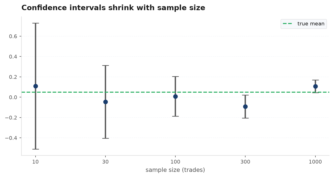
Many repeated-sample confidence intervals plotted vertically around the true parameter, most covering it and a few missing — Coverage is a property of the procedure, not of any single interval: across repeated samples, about 95% of the intervals catch the fixed true value and 5% miss. Your one realised interval either contains it or it doesn't — there is no 95% probability left once the data are in.

!CI interpretation traps

“There is a 95% probability that $μ$ lies in $[2.1, 4.3]$ ” is wrong in the frequentist framework: $μ$ is a fixed number and the realised interval is fixed too — the coverage probability belongs to the procedurebefore the data arrive. The statement quants actually want (“given my data, where is the parameter probably?”) is a credible interval, which requires a prior — the central topic of Bayesian inference. Also: a CI is not a range of plausible data, not a prediction interval for the next observation, and 95% of sample points do not fall inside it.

Power and sample size#

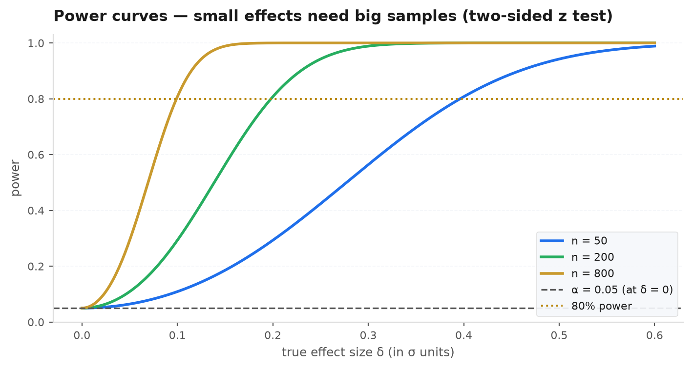
Power is where testing meets budgeting: how much data buys a given probability of detecting a given effect? For the two-sided z-test the whole calculation is three lines.

✦Derivation — the sample-size formula

Reject when $∣ X ˉ - μ_{0} ∣ > z_{α /2} σ / n$ . Suppose the truth is $μ_{0} + δ$ with $δ > 0$ . Then $Z = (X ˉ - μ_{0} - δ) / (σ / n)$ is standard normal, and (neglecting the far tail) the power is

1 - β \approx P (Z > z_{α /2} - \frac{δ n}{σ}) = Φ (\frac{δ n}{σ} - z_{α /2}) .

Setting this equal to $1 - β$ gives $δ n / σ - z_{α /2} = z_{β}$ , i.e.

n = (\frac{( z _{α /2} + z _{β} ) σ}{δ})^{2} .

The two constants to memorise: $z_{0.025} = 1.96$ and $z_{0.20} = 0.84$ , so 80% power at 5% two-sided needs $n = (2.80 σ / δ)^{2} \approx 7.85 (σ / δ)^{2}$ . Note the brutal scaling: halving the detectable effect quadruples the required sample.

Worked numeric: to detect a shift of $δ = 0.5 σ$ with 80% power at 5%: $n = (2.80/0.5)^{2} \approx 31.4 \to 32$ . To detect $δ = 0.1 σ$ : $n = 784$ . And the coin from earlier: to detect $p = 0.55$ vs 0.5 (a $δ / σ \approx 0.1$ effect per flip), you need roughly 780 flips — 100 was never going to settle it.

Power curves as a function of true effect size for several sample sizes, all passing through alpha at zero effect and rising toward one — Power curves: probability of rejecting as a function of the true effect, for several n. Every curve starts at alpha (the false-positive rate at zero effect) and rises; larger samples rise faster. The dashed 80% line marks the conventional design target — find where your curve crosses it.

→Quant lens — the t-stat of a strategy, and why a year proves nothing

A backtest’s headline test is a one-sample t on mean trade (or daily) return. With $T$ daily observations, $t = r ˉ / (s / T) = SR_{daily} T$ , and since $SR_{ann} = SR_{daily} 252$ ,

t \approx SR_{ann} \times years .

A true Sharpe-1 strategy observed for one year has expected t-stat 1.0 — far below 1.96. Its power at the 5% level is $Φ (1 - 1.96) \approx 17%$ : five times out of six, a genuinely good strategy fails the significance test on a year of data. For 80% power you need $years \geq 2.80$ , i.e. about 8 years. Equivalently, 200 trades averaging 0.08R with spread 1.1R give $t = 0.08/ (1.1/ 200) \approx 1.03$ — you would need roughly 730 trades at that edge for significance. This arithmetic — not pessimism — is why the gauntlet demands long samples and why small edges need hundreds of independent bets to be distinguishable from luck.

The peeking problem#

The level- $α$ guarantee assumes the sample size was fixed in advance. If instead you test after every new observation and stop when $p < 0.05$ , the true false-positive rate inflates far beyond 5% — by the law of the iterated logarithm, the running t-statistic crosses any fixed boundary eventually with probability 1 under the null. Peeking is optional stopping used against yourself (compare optional stopping: no stopping rule beats a fair game, but a stopping rule can absolutely beat a naive significance threshold).

peeking_inflates_alpha.py

import numpy as np

rng = np.random.default_rng(11)
n_paths, n_max = 2000, 500
ever, fixed_n = 0, 0
for _ in range(n_paths):
    x = rng.standard_normal(n_max)            # H0 true: mean is exactly 0
    n = np.arange(1, n_max + 1)
    mean = np.cumsum(x) / n
    var = (np.cumsum(x**2) - n * mean**2) / np.maximum(n - 1, 1)
    t = np.abs(mean / np.sqrt(var / n))
    ever += np.any(t[9:] > 1.96)              # peek at every n >= 10
    fixed_n += t[-1] > 1.96                   # single test at n = 500
print(f"reject once at n=500:   {fixed_n / n_paths:.3f}")   # ~0.05, as designed
print(f"reject if peeking:      {ever / n_paths:.3f}")      # ~0.28 -- 5x inflation

The honest fixed-n test rejects about 5% of the time; the peeker rejects nearly 30% of the time on pure noise. The same mechanism operates when a researcher re-runs a backtest after each tweak and stops at the first significant variant — that is peeking across model space rather than time, and it is the subject of multiple testing & paradoxes. Sequential designs that permit peeking honestly (alpha-spending, always-valid inference) exist, but they pay with wider boundaries.

Finally, keep statistical and practicalsignificance separate. With enough data, a strategy earning 0.2 basis points per trade will be statistically significant — and still die to transaction costs. The test answers “is the effect distinguishable from zero?”, never “is the effect big enough to matter?”. Report effect sizes with intervals, not verdicts.

Practice problems#

→Problem 1 — interpret p = 0.04

A backtest of a signal yields p = 0.04 against the no-edge null. Your PM asks: “so there’s a 96% chance this signal is real?” Respond precisely.

Solution. No. The correct statement: if the signal had no edge, the probability of seeing a result at least this strong is 4%. It is $P (data ∣ H_{0})$ -flavoured, not $P (H_{0} ∣ data)$ . Converting to the PM’s question needs a prior: by Bayes, $posterior odds = prior odds \times Bayes factor$ , and the bound $BF \leq 1/ (- e p ln p) \approx 2.9$ at p = 0.04 means the evidence multiplies the odds by at most ~3. If only ~10% of tested signals are real (prior odds 1:9), the posterior probability of a real edge is at most about $3/ (3 + 9) = 25%$ — and if this was the best of many variants tried, the p-value itself is invalid before we even start (multiple testing).

→Problem 2 — 60 heads in 100 flips

Is the coin biased? Give the test, the number, and the decision — then say how many flips you would want.

Solution. Two-sided binomial test. Normal approximation: $z = (60 - 50) / 100 \cdot 0.25 = 2.0$ , p ≈ 0.046; with continuity correction z = 1.9, p ≈ 0.057; exact p ≈ 0.057. Borderline — the honest answer is “weak evidence of bias, not conclusive.” Follow-up: to reliably detect a coin with p = 0.6 (80% power, 5% level), $n = ((1.96 + 0.84) σ / δ)^{2}$ with $δ = 0.1$ , $σ \approx 0.5$ per flip: $n \approx (2.80 \times 5)^{2} = 196$ flips. The slick closing check: the observed 2-sigma result is exactly what a fair coin produces one time in twenty.

→Problem 3 — power to detect Sharpe 1 in one year

A strategy truly has annualised Sharpe 1. You observe one year of daily returns and run a 5% two-sided t-test of zero mean. What is the power? How long until 80%?

Solution. The t-statistic’s noncentrality is $SR_{daily} 252 = SR_{ann} years = 1$ . Power $\approx P (Z > 1.96 - 1) = Φ (- 0.96) \approx 17%$ (the other tail is negligible). For 80% power, need noncentrality $1.96 + 0.84 = 2.80$ , so $years = 2.80 \Rightarrow\approx 7.8$ years. Moral: a year of live trading cannot statistically validate even a genuinely excellent strategy — which is why allocators look at process, capacity, and out-of-sample behaviour rather than one-year track records.

→Problem 4 — a CI for the difference of two strategies

Strategy A: mean daily return 0.08%, sd 1.2%, n = 252. Strategy B: mean 0.02%, sd 1.0%, n = 252 (independent). Give a 95% CI for the difference in means and the test verdict.

Solution. The difference is 0.06% with standard error

se = \frac{1. 2 ^{2}}{252} + \frac{1. 0 ^{2}}{252} = \frac{2.44}{252} \approx 0.098%.

CI: $0.06 \pm 1.96 \times 0.098 = [- 0.13%, + 0.25%]$ . Zero is comfortably inside — by the duality above, the 5% test does not reject equal means (t ≈ 0.61). Two refinements earn bonus points: (i) if A and B trade the same market their returns are correlated, so the paired test on daily differences is correct and usually much sharper (the covariance term subtracts); (ii) daily autocorrelation shrinks the effective n, widening the honest interval (time-series statistics).

→Problem 5 — why 1.96?

Where does 1.96 come from, and what are its 90% and 99% siblings?

Solution. A two-sided 5% test splits $α$ into 2.5% per tail, so the threshold is the 97.5th percentile of the standard normal: $Φ (z) = 0.975 \Rightarrow z = 1.96$ . It is a property of the Gaussian CDF, nothing deeper — and it is only correct insofar as the CLT normal approximation holds for your statistic. Siblings: $z_{0.05} = 1.645$ (90% two-sided or 95% one-sided), $z_{0.005} = 2.576$ (99%). Fat-tailed or autocorrelated returns break the 1.96 calibration: the true 97.5th percentile of a t(4)-ish return distribution’s mean at modest n is noticeably wider, which is one reason bootstrap intervals are preferred for Sharpe-type statistics.

Next:the p-value chapter’s recurring complaint — “what I actually want is the probability of the hypothesis given the data” — has an answer, and it costs a prior. Bayesian inference.