Bayesian inference

The frequentist chapter kept insisting that a p-value is not the probability the hypothesis is true. Bayesian inference is the framework in which that probability exists: treat the unknown parameter as a random variable, encode what you believed before the data as a prior, and let Bayes’ theorem convert data into an updated belief. This chapter derives — not merely states — the three classic conjugate updates (beta–binomial, normal–normal, gamma–Poisson), pins down exactly how credible intervals differ from confidence intervals, and connects posterior means, MAP, and MLE through loss functions.

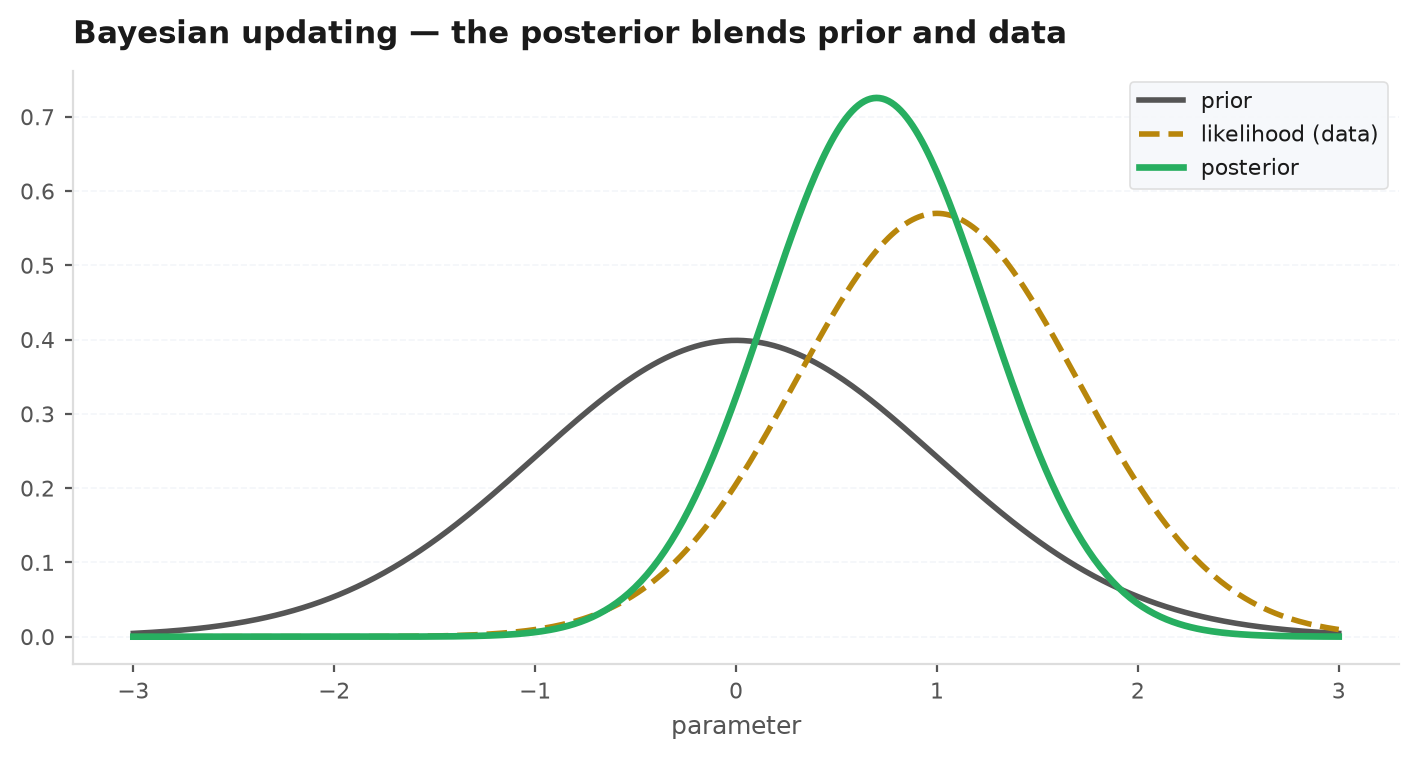
✦Intuition — inference as bookkeeping on beliefs

You already reason this way at the desk. You believe a strategy has a small edge (prior). It wins seven of its next ten trades (likelihood). You now believe in it a bit more — but not as much as the raw 70% hit rate suggests, because ten trades is nothing (posterior: a compromise, weighted by how much information each side carries). Bayes’ theorem is the unique consistent arithmetic for that compromise. The entire chapter is one identity applied relentlessly: $posterior \propto likelihood \times prior$ , with the normalising constant left to fend for itself.

Bayes for parameters#

Let $θ$ be the unknown parameter and $x$ the data. The four objects of Bayesian inference:

posterior p (θ ∣ x) = \frac{p ( x ∣ θ ) likelihood p ( θ ) prior}{evidence p ( x )}, p (x) = \int p (x ∣ θ) p (θ) d θ .

The evidence $p (x)$ is a constant in $θ$ , so in practice you work with $p (θ ∣ x) \propto p (x ∣ θ) p (θ)$ and normalise at the end — the engine of every derivation below. Two structural properties fall out immediately:

Sequential updating.Today’s posterior is tomorrow’s prior. Processing observations one at a time, or all at once, gives the identical posterior — multiply the likelihoods and the order of multiplication cannot matter. Bayesian learning is streaming by construction.
Prediction. The posterior predictive for a new observation averages the model over remaining parameter uncertainty: $p (x ~ ∣ x) = \int p (x ~ ∣ θ) p (θ ∣ x) d θ$ — fatter-tailed than any single- $θ$ forecast, because it prices in not knowing $θ$ .

A sequence of posterior densities for a coin's heads probability, starting flat and sharpening around the true value as flips accumulate — Sequential Bayesian updating: a flat prior over a coin's heads probability sharpens flip by flip. Each posterior becomes the next prior; the batch answer and the one-at-a-time answer coincide exactly. Information accumulates as the density narrows — the Bayesian picture of the law of large numbers.

Conjugacy I — beta–binomial, derived#

A prior is conjugateto a likelihood when the posterior stays in the prior’s family — updating reduces to updating a few hyperparameters. The workhorse example: a coin (a trade’s win indicator) with unknown heads probability $θ$ .

✦Derivation — Beta prior + binomial data ⇒ Beta posterior

Take prior $θ \sim Beta (a, b)$ , density $p (θ) \propto θ^{a - 1} (1 - θ)^{b - 1}$ , and observe $k$ heads in $n$ flips, likelihood $p (k ∣ θ) \propto θ^{k} (1 - θ)^{n - k}$ . Multiply and keep only $θ$ -dependence:

p (θ ∣ k) \propto θ^{k} (1 - θ)^{n - k} \cdot θ^{a - 1} (1 - θ)^{b - 1} = θ^{a + k - 1} (1 - θ)^{b + n - k - 1} .

That is precisely the kernel of a Beta density, so — no integration required —

θ ∣ k \sim Beta (a + k, b + n - k) .

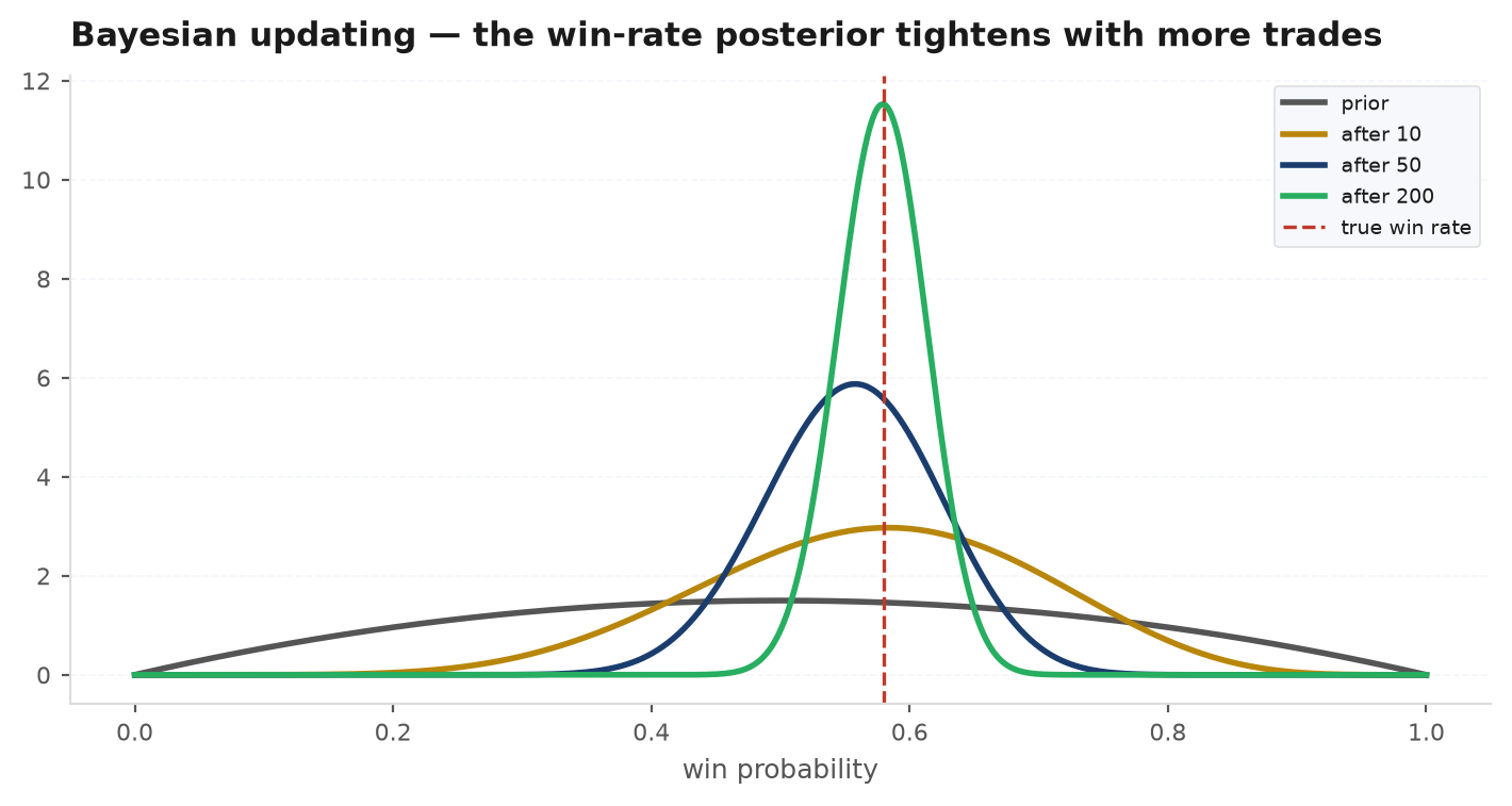
The hyperparameters act as pseudo-counts: the prior behaves like $a$ imaginary heads and $b$ imaginary tails already seen. The posterior mean exposes the compromise explicitly:

E [θ ∣ k] = \frac{a + k}{a + b + n} = w_{prior} \frac{a + b}{a + b + n} \cdot \frac{a}{a + b} + w_{data} \frac{n}{a + b + n} \cdot \frac{k}{n} .

A weighted average of prior mean and sample frequency, with weights proportional to pseudo-counts vs real counts. As $n \to \infty$ the data weight tends to 1 and the posterior mean approaches the MLE $k / n$ — priors wash out under data.

Worked numeric: prior $Beta (2, 2)$ (mean 0.5, worth 4 pseudo-flips), observe 7 wins in 10 trades. Posterior: $Beta (9, 5)$ , mean $9/14 \approx 0.643$ — pulled from the raw 0.700 toward 0.5 by exactly the ratio $4/14$ of pseudo-data to total data. Posterior standard deviation $9 \cdot 5/ (1 4^{2} \cdot 15) \approx 0.124$ : the hit rate is known to roughly ±12% — still very little.

Beta prior, scaled binomial likelihood, and resulting Beta posterior for a coin's heads probability on one axis — Beta prior, binomial likelihood, Beta posterior — the conjugate triangle. The posterior sits between prior and likelihood, closer to whichever carries more effective observations. With pseudo-counts a + b = 4 against n = 10 real flips, the data get 10/14 of the vote.

Conjugacy II — normal–normal and precision weighting#

Now estimate a mean — a strategy’s true daily edge $θ$ — from $n$ observations $x_{i} \sim N (θ, σ^{2})$ with $σ^{2}$ known, and prior $θ \sim N (μ_{0}, τ_{0}^{2})$ . Define precision = 1/variance; the result is cleanest in that currency.

✦Derivation — complete the square, get precision-weighted shrinkage

The likelihood depends on the data only through $x ˉ \sim N (θ, σ^{2} / n)$ . The log-posterior is, up to constants,

lo g p (θ ∣ x ˉ) = - \frac{( θ - μ _{0} ) ^{2}}{2 τ _{0}^{2}} - \frac{n ( θ - x ˉ ) ^{2}}{2 σ ^{2}} + const .

Expand and collect the quadratic and linear terms in $θ$ :

lo g p (θ ∣ x ˉ) = - \frac{1}{2} (\frac{1}{τ _{0}^{2}} + \frac{n}{σ ^{2}}) θ^{2} + (\frac{μ _{0}}{τ _{0}^{2}} + \frac{n x ˉ}{σ ^{2}}) θ + const .

A quadratic log-density is a Gaussian, with precision equal to the coefficient of $- θ^{2} /2$ and mean equal to (linear coefficient)/(precision):

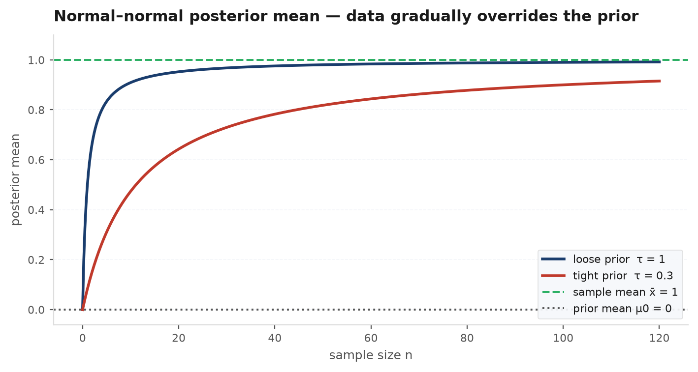
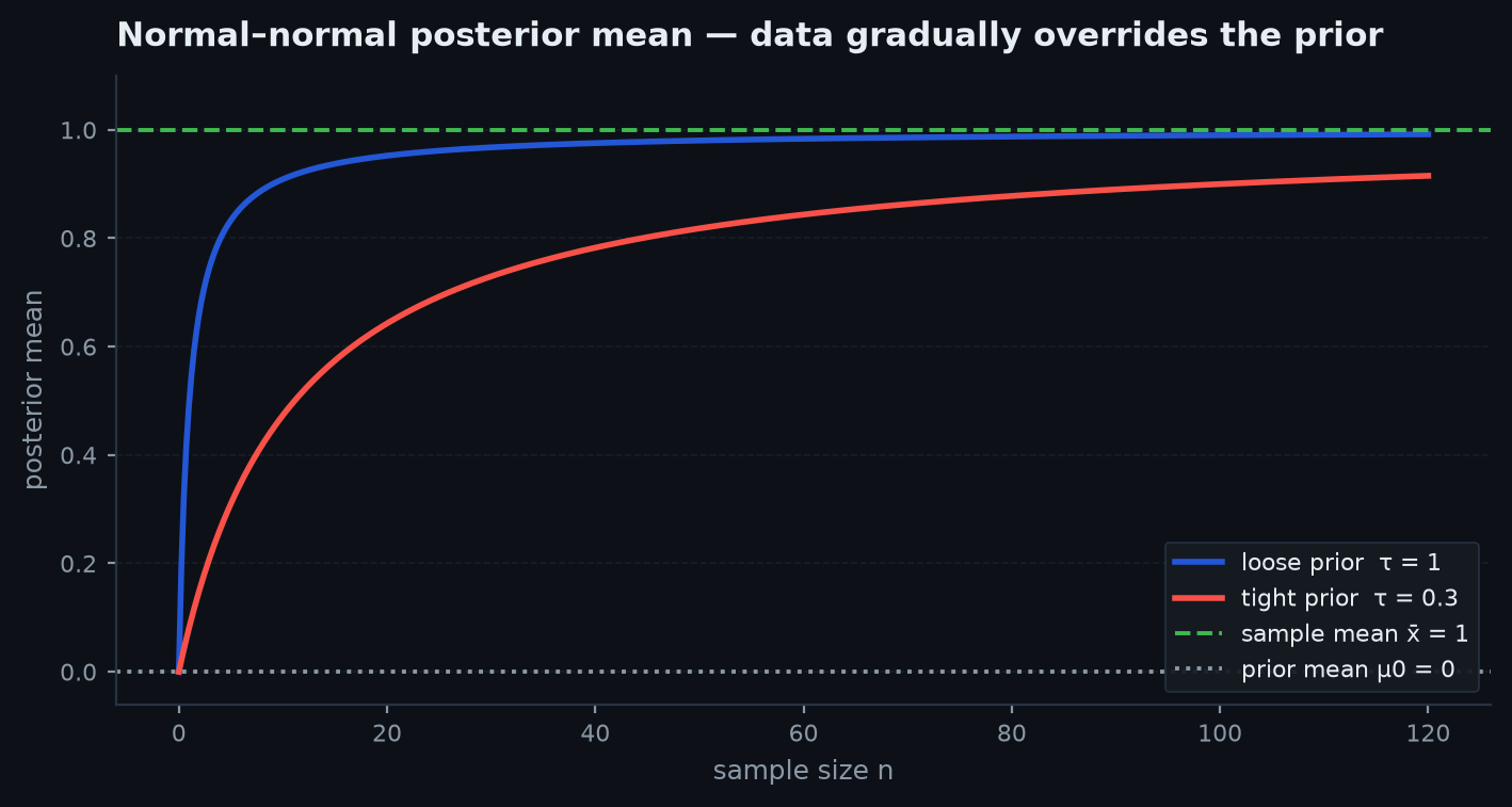
θ ∣ x ˉ \sim N (μ_{1}, τ_{1}^{2}), \frac{1}{τ _{1}^{2}} = \frac{1}{τ _{0}^{2}} + \frac{n}{σ ^{2}}, μ_{1} = \frac{\frac{μ _{0}}{τ _{0}^{2}} + \frac{n x ˉ}{σ ^{2}}}{\frac{1}{τ _{0}^{2}} + \frac{n}{σ ^{2}}} .

Read it twice. Precisions add: certainty accumulates linearly in information. And the posterior mean is a precision-weighted average of prior mean and sample mean — each source of information votes in proportion to how sure it is. Writing $w = τ_{0}^{2} / (τ_{0}^{2} + σ^{2} / n)$ , the mean is $μ_{1} = w x ˉ + (1 - w) μ_{0}$ : the data estimate shrunk toward the priorby a factor determined by relative noise. This is the same shrinkage that reappears as James–Stein and empirical Bayes in estimators & sampling, and as beta shrinkage in regression.

Worked numeric: prior $θ \sim N (0, 2^{2})$ (edge probably near zero), data $x ˉ = 1.2$ with $σ^{2} / n = 1$ . Posterior precision $= 1/4 + 1 = 1.25$ , so $τ_{1}^{2} = 0.8$ ; posterior mean $= (0 \times 0.25 + 1.2 \times 1) /1.25 = 0.96$ . The data are four times as precise as the prior, so the estimate moves 80% of the way from 0 to 1.2.

Prior, likelihood, and posterior Gaussians on one axis, with the posterior mean visibly between the prior and sample means, weighted toward the sharper density — Normal-normal updating: the posterior Gaussian sits between prior and likelihood, its mean the precision-weighted average and its precision the sum. The sharper curve pulls harder. Shrinkage is not a correction bolted on afterwards — it is what Bayes' theorem computes.

Conjugacy III — gamma–Poisson#

For count data — order arrivals, jump counts (Poisson processes) — with rate $λ$ : take prior $λ \sim Gamma (a, b)$ (shape $a$ , rate $b$ ), density $\propto λ^{a - 1} e^{- bλ}$ , and observe counts $x_{1}, \dots, x_{n}$ with likelihood $\propto λ^{\sum x_{i}} e^{- nλ}$ . Multiplying kernels:

p (λ ∣ x) \propto λ^{a + \sum x_{i} - 1} e^{- (b + n) λ} ⟹ λ ∣ x \sim Gamma (a + \sum x_{i}, b + n) .

Posterior mean $(a + \sum x_{i}) / (b + n)$ : again pseudo-data — the prior is worth $a$ events over $b$ periods, blended with the observed $\sum x_{i}$ events over $n$ periods. Worked numeric: a desk believes a venue sends roughly 20 fills/hour, worth two hours of pseudo-observation: $Gamma (40, 2)$ . Watching 3 hours with 45 fills gives posterior $Gamma (85, 5)$ , mean 17/hour, sd $85 /5 \approx 1.84$ . The three conjugate families share one grammar:

Likelihood	Conjugate prior	Posterior update	Pseudo-data reading
Binomial(n, θ)	Beta(a, b)	Beta(a + k, b + n − k)	a heads, b tails already seen
Normal(θ, σ² known)	Normal(μ₀, τ₀²)	precision-weighted Normal	prior ≈ σ²/τ₀² extra observations
Poisson(λ)	Gamma(a, b)	Gamma(a + Σx, b + n)	a events over b periods

Credible vs confidence intervals — the exact difference#

A $95%$ credible interval is a set with posterior probability 0.95: $P (θ \in C ∣ x) = 0.95$ — a direct probability statement about the parameter, given your data and prior. A confidence interval makes a coverage promise about the procedure across hypothetical repetitions: $P_{θ} (θ \in C (X)) = 0.95$ before the data arrive. With flat priors and no constraints the two often coincide numerically, which breeds the confusion. They split apart the moment real prior information exists — most vividly, a support constraint:

✦Worked example — where the two intervals genuinely differ

Suppose $θ \geq 0$ is known (a variance, a capacity, a squared quantity), and one observation $x \sim N (θ, 1)$ lands at $x = - 1.0$ . The standard 95% confidence interval is

x \pm 1.96 = [- 2.96, 0.96],

which is mostly impossible values — and had $x = - 2.5$ occurred, the interval $[- 4.46, - 0.54]$ would contain no feasible value at all, while the procedure still boasts 95% coverage (it fails only in the 5% of samples like this one). The Bayesian answer with a flat prior on $[0, \infty)$ is the truncated normal $p (θ ∣ x) \propto φ (θ + 1) 1 {θ \geq 0}$ . Its equal-tailed 95% credible interval solves $Φ (θ + 1) = Φ (1) + q (1 - Φ (1))$ at $q = 0.025, 0.975$ , giving approximately

[0.02, 1.65] .

Every value is feasible, and the interval concentrates just above zero — exactly what the evidence plus the constraint warrant. The confidence procedure is calibrated on average over samples; the credible interval is calibrated for the sample you actually have. A crisp way to phrase it: “the CI answers a question about the method, the credible interval answers a question about the parameter.”

Point estimates as loss functions — MAP vs MLE vs posterior mean#

Collapsing a posterior to one number is a decision, and decisions need a loss. Choosing the estimate $a$ to minimise expected posterior loss gives:

Squared loss ⇒ posterior mean. $\frac{d}{d a} E [(θ - a)^{2} ∣ x] = - 2 E [θ - a ∣ x] = 0$ gives $a = E [θ ∣ x]$ — the same L2-optimality as conditional expectation in joint distributions.
Absolute loss ⇒ posterior median. Balancing probability mass on each side.
0–1 loss ⇒ MAP (posterior mode), the limit of rewarding only near-exact hits. And since $ar g max_{θ} p (θ ∣ x) = ar g max_{θ} p (x ∣ θ) p (θ)$ , MAP with a flat prior is exactly the MLE of the previous part. A Gaussian prior turns MAP into ridge regression; a Laplace prior into lasso — regularisation is a prior in disguise.

For skewed posteriors the three disagree materially: in the Beta(9,5) example, mean 0.643, mode $8/12 \approx 0.667$ , median $\approx 0.647$ . For the heavy-tailed German-tank posterior in Problem 5, mean and median differ by 40%.

Priors — choice, Jeffreys, and sensitivity#

The prior is the framework’s cost of admission. Practical guidance:

Flat is not innocent. A uniform prior on $θ$ is not uniform on $θ^{2}$ or $lo g θ$ — “no information” is parameterisation-dependent. The Jeffreys prior $π (θ) \propto I (θ)$ (Fisher information from Cramér–Rao) fixes this by being invariant under reparameterisation; for a Bernoulli it is $Beta (\frac{1}{2}, \frac{1}{2})$ .
Sensitivity fades as $n$ grows. The data weight in every conjugate update above is $n / (n + n_{pseudo})$ ; report posterior conclusions under two or three plausible priors and show they agree before trusting them.
Empirical Bayes teaser. With many parallel problems (5,000 strategies, each with a hit rate), estimate the prior from the ensembleand shrink each estimate toward it — the James–Stein phenomenon operationalised. This is the statistically honest version of “compare each strategy to the population of strategies you tried.”

Checking a derivation by simulation#

Conjugacy claims are exactly checkable: sample $θ$ from the prior, simulate data, keep the draws whose simulated data match the observed data. The surviving draws are samples from the posterior (this is rejection ABC — and the definition of conditioning). Verifying $Beta (2, 2) + 7/10 \Rightarrow Beta (9, 5)$ :

conjugacy_check.py

import numpy as np

rng = np.random.default_rng(11)
a, b, n, k = 2.0, 2.0, 10, 7

theta = rng.beta(a, b, size=2_000_000)     # draws from the prior
sims = rng.binomial(n, theta)              # each theta flips its own coin
post = theta[sims == k]                    # condition on the observed data

exact_mean = (a + k) / (a + b + n)         # Beta(9,5) mean = 0.6429
exact_var = ((a + k) * (b + n - k)) / ((a + b + n) ** 2 * (a + b + n + 1))
print(f"accepted draws:   {post.size}")
print(f"posterior mean:   {post.mean():.4f}   exact {exact_mean:.4f}")
print(f"posterior var:    {post.var():.5f}  exact {exact_var:.5f}")
print(f"P(theta > 0.5):   {(post > 0.5).mean():.4f}")

The empirical mean and variance land on the Beta(9,5) values to three decimals, and you get $P (θ > 0.5 ∣ data) \approx 0.85$ for free — the probability the strategy is better than a coin, a number no p-value will ever hand you.

→Quant lens — Kelly under parameter uncertainty, regimes, and Thompson

Three places this machinery earns money. (1) Sizing. Kelly says bet $f^{*} = 2 p - 1$ of bankroll on an even-money edge — but you never know $p$ , only a posterior. Maximising expected log growth over the posterior predictive shrinks the bet: uncertainty about the edge behaves like extra variance, and overbetting an overestimated edge is ruinous while underbetting is merely slow (see bandits & allocation). Fractional Kelly is an informal posterior shrinkage. (2) Regimes. Beliefs about the current market state update by exactly the sequential Bayes rule above — the filter behind regime detection is this chapter running in a loop. (3) Exploration.Thompson sampling allocates capital to strategies by sampling each one’s posterior and backing the sampled winner — randomised exactly in proportion to the probability each strategy is best. See Bayesian methods for the applied toolkit.

Practice problems#

→Problem 1 — posterior for a biased coin

With a uniform prior on $θ$ , a coin shows 7 heads in 10 flips. Give the posterior, its mean, its mode, and the probability the next flip is heads.

Solution. Uniform = Beta(1,1), so the posterior is $Beta (1 + 7, 1 + 3) = Beta (8, 4)$ . Mean $8/12 = 2/3$ ; mode $(8 - 1) / (8 + 4 - 2) = 0.7$ — equal to the MLE, as it must be under a flat prior. The predictive probability of heads is the posterior mean, $2/3$ , not 0.7: prediction integrates over uncertainty rather than plugging in the best guess, and the integral drags the answer toward 1/2. Distinguishing those two numbers crisply is the point of the question.

→Problem 2 — Laplace's rule of succession

Derive: after observing $k$ successes in $n$ trials with a uniform prior, the probability the next trial succeeds is $(k + 1) / (n + 2)$ .

Solution. Posterior is $Beta (k + 1, n - k + 1)$ by the beta–binomial derivation. The predictive is its mean:

P (success ∣ data) = E [θ ∣ data] = \frac{k + 1}{( k + 1 ) + ( n - k + 1 )} = \frac{k + 1}{n + 2} .

The +1/+2 are the flat prior’s pseudo-counts (one imagined success, one imagined failure). Note the consequences: after n successes in n trials the answer is $(n + 1) / (n + 2) < 1$ — a Bayesian never assigns probability 1 from finite data — and with n = 0 the rule gives 1/2. A strategy that is 3-for-3 has predictive win rate 4/5, not 1.

→Problem 3 — a normal-normal update by hand

Prior: $θ \sim N (0, 4)$ . You observe a sample mean of 1.2 with sampling variance 1. Posterior?

Solution. Work in precisions: prior 1/4, data 1. Posterior precision $= 0.25 + 1 = 1.25 \Rightarrow$ variance $0.8$ . Posterior mean = precision-weighted average:

μ_{1} = \frac{0.25 \times 0 + 1 \times 1.2}{1.25} = 0.96, θ ∣ x \sim N (0.96, 0.8) .

Sanity checks worth stating explicitly: the posterior mean lies between 0 and 1.2, closer to the data (which are 4× more precise); the posterior variance (0.8) is smaller than boththe prior’s (4) and the data’s (1), because precisions add.

→Problem 4 — would one more win change your mind?

A strategy has won 55 of 100 trades (uniform prior). It wins the next trade. How much does your estimate of its hit rate move? What if it had only ever traded twice, winning both?

Solution. Before: Beta(56, 46), mean $56/102 \approx 0.549$ . After: Beta(57, 46), mean $57/103 \approx 0.553$ — a move of 0.4%. In general one observation moves the posterior mean by $O (1/ n)$ : with n = 100 the belief is stiff. With 2-for-2, the mean jumps from $3/4$ to $4/5$ — 5 points — because the posterior is still wide. The key point: the same evidence moves beliefs by an amount inversely proportional to the information already held; anyone who re-sizes positions dramatically on one good week is running an n-of-5 posterior on an n-of-500 problem.

→Problem 5 — Bayesian German tank

You see serial numbers 17, 42, 60 from a fleet numbered 1..N. With a flat prior on N, estimate N. Why do the posterior mean and median disagree so much?

Solution. The likelihood of observing 3 particular distinct serials is $(3 N)^{- 1} \propto N^{- 3}$ (approximately) for $N \geq 60$ , zero below. With a flat prior, the posterior is $\propto N^{- 3}$ on $[60, \infty)$ — a power law. Continuous approximation with $m = 60, n = 3$ :

E [N ∣ data] \approx m \frac{n - 1}{n - 2} = 120, median = m \cdot 2^{1/ (n - 1)} \approx 85.

The frequentist UMVU estimate $m (1 + 1/ n) - 1 = 79$ (see estimators) sits near the posterior median, while the posterior mean is dragged to 120 by the heavy right tail — enormous fleets are improbable but not impossible, and squared loss cares about them. The disagreement is the loss-function lesson of this chapter in one number: report the median (or the whole posterior) when tails are heavy, and know which loss your estimate is optimising before you quote it.

Next: from beliefs about single parameters to the workhorse of empirical finance — fitting lines through noise, and knowing precisely when to trust the fitted slope. Regression & Gauss–Markov.