Estimators & sampling theory

Every number you compute from data — a mean return, a volatility, a Sharpe ratio — is an estimator: a random variable whose value would have been different on a different sample. Statistical inference begins by taking that randomness seriously: what distribution does the estimator itself follow, is it aimed at the right target (bias), how much does it scatter (variance), and is there a floor on how precise any estimator can be (Cramér–Rao)? This chapter builds the machinery: MSE decomposition, the story behind $n - 1$ , the genesis of the $t$ distribution, Fisher information, and sufficiency.

✦Intuition — the estimator is a random variable

Fix a model: data $X_{1}, \dots, X_{n}$ drawn iid from a distribution with unknown parameter $θ$ . A statistic is any function of the data $T (X_{1}, \dots, X_{n})$ ; an estimator is a statistic used to guess $θ$ . Because the data are random, $T$ has its own distribution — the sampling distribution — and every question about estimation quality is a question about that distribution: where is it centred, how wide is it, what shape does it take as $n$ grows. The single most common conceptual failure is treating an estimate as a number rather than a draw.

Bias, variance, and mean squared error#

For an estimator $θ^$ of $θ$ , define the bias $b (θ^) = E [θ^] - θ$ and the mean squared error $MSE (θ^) = E [(θ^- θ)^{2}]$ . These connect through the fundamental decomposition:

MSE (θ^) = Var (θ^) + b (θ^)^{2} .

✦Proof — bias–variance decomposition

Add and subtract $μ_{T} := E [θ^]$ inside the square:

E [(θ^- θ)^{2}] = E [(θ^- μ_{T})^{2}] + 2 E [θ^- μ_{T}] (μ_{T} - θ) + (μ_{T} - θ)^{2} .

The cross term vanishes because $E [θ^- μ_{T}] = 0$ and $μ_{T} - θ$ is a constant. What remains is variance plus squared bias. Moral: unbiasedness is not sacred — a small bias is a good trade if it buys a large variance reduction. Shrinkage estimators live on exactly this trade.

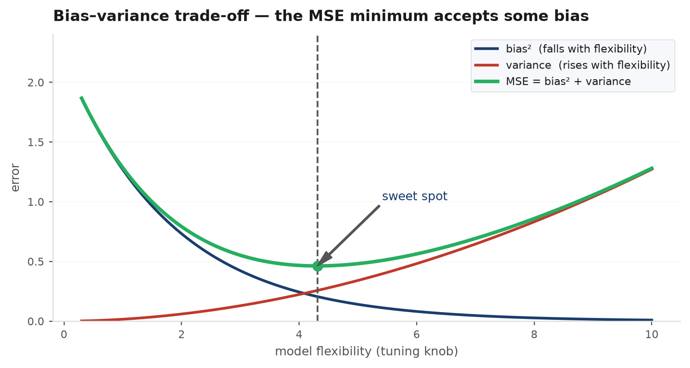
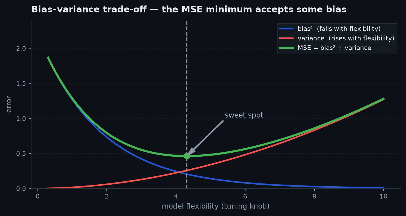
Sampling distributions of a biased low-variance estimator and an unbiased high-variance estimator around the true parameter, showing the biased one can have lower MSE — Two sampling distributions for the same target. The unbiased estimator is centred on the truth but wide; the biased one is slightly off-centre but tight. MSE = variance + bias^2 scores the whole picture — and the biased estimator can win.

Two more properties complete the vocabulary. $θ^_{n}$ is consistent if $θ^_{n} \to θ$ in probability as $n \to \infty$ — by Chebyshev (see inequalities & bounds), it suffices that bias and variance both vanish. $θ^$ is efficientif its variance attains the Cramér–Rao lower bound below. Consistency is a minimal sanity requirement (more data should get you there); efficiency is the gold standard at finite $n$ .

Worked example. Estimate $σ^{2}$ of a normal from $n = 10$ observations with true $σ^{2} = 4$ , using $S_{c} = c \sum_{i} (X_{i} - X ˉ)^{2}$ . Since $\sum (X_{i} - X ˉ)^{2} \sim σ^{2} χ_{9}^{2}$ (mean 9, variance 18), the divisor $n - 1 = 9$ gives bias 0 and MSE $2 σ^{4} /9 \approx 3.56$ ; the divisor $n = 10$ gives bias $- 0.4$ and MSE $3.04$ ; the divisor $n + 1 = 11$ gives bias $- 0.73$ and MSE $2 σ^{4} /11 \approx 2.91$ — the most biased of the three has the lowest MSE. Problem 1 below proves $1/ (n + 1)$ is optimal in this class.

Why s² divides by n − 1#

The sample variance is $s^{2} = \frac{1}{n - 1} \sum_{i = 1}^{n} (X_{i} - X ˉ)^{2}$ . The $n - 1$ exists because the deviations are measured from $X ˉ$ , which was itself fit to the data — the sample mean chases the sample, making raw squared deviations systematically too small.

✦Proof — E[s²] = σ²

Decompose deviations about $μ$ into deviations about $X ˉ$ plus the mean’s own error (the cross term telescopes to zero):

i \sum (X_{i} - μ)^{2} = i \sum (X_{i} - X ˉ)^{2} + n (X ˉ - μ)^{2} .

Take expectations: the left side is $n σ^{2}$ , and $E [n (X ˉ - μ)^{2}] = n \cdot σ^{2} / n = σ^{2}$ . Hence

E [i \sum (X_{i} - X ˉ)^{2}] = n σ^{2} - σ^{2} = (n - 1) σ^{2},

so dividing by $n - 1$ is exactly what restores unbiasedness. One degree of freedom was spent estimating $μ$ ; the correction refunds it.

Hand computation: data ${1, 3, 5}$ gives $X ˉ = 3$ and $\sum (X_{i} - X ˉ)^{2} = 4 + 0 + 4 = 8$ , so $s^{2} = 8/2 = 4$ , while the $1/ n$ version gives $8/3 \approx 2.67$ — smaller, as the bias predicts.

!s is still biased for σ

Unbiasedness does not survive nonlinear transformations. Since $Var (s) = E [s^{2}] - (E [s])^{2} > 0$ whenever $s$ is non-degenerate, $(E [s])^{2} < σ^{2}$ , i.e. $E [s] < σ$ : the sample standard deviation systematically understates volatility. This is Jensen’s inequality for the strictly concave square root (see Jensen). Under normality the exact correction is known (about $1 + 1/ (4 n)$ ), but the point to internalise is the direction and the reason.

Sampling distributions under normality#

Let $X_{1}, \dots, X_{n} \sim N (μ, σ^{2})$ iid. Three exact facts organise all of classical inference:

$X ˉ \sim N (μ, σ^{2} / n)$ — exactly, not just asymptotically (linear combinations of normals are normal: joint distributions).
$(n - 1) s^{2} / σ^{2} \sim χ_{n - 1}^{2}$ — a sum of squares of $n - 1$ effective standard normals, one degree lost to $X ˉ$ .
$X ˉ$ and $s^{2}$ are independent — a property that characterises the normal distribution.

✦Proof sketch — independence and the genesis of t

Sketch of independence: the vector of deviations $(X_{1} - X ˉ, \dots, X_{n} - X ˉ)$ and $X ˉ$ are jointly normal, and $Cov (X_{i} - X ˉ, X ˉ) = σ^{2} / n - σ^{2} / n = 0$ ; for jointly Gaussian vectors zero covariance implies independence, and $s^{2}$ is a function of the deviations alone. Now define a $t$ variable with $k$ degrees of freedom as $T = Z / V / k$ with $Z \sim N (0, 1)$ independent of $V \sim χ_{k}^{2}$ . Then

\frac{X ˉ - μ}{s / n} = \frac{( X ˉ - μ ) / ( σ / n )}{[ ( n - 1 ) s ^{2} / σ ^{2} ] / ( n - 1 )} \sim t_{n - 1},

because the numerator is standard normal, the bracket is $χ_{n - 1}^{2}$ , and the two are independent. Every unknown- $σ$ test and confidence interval in hypothesis testing is this one algebraic identity. The extra randomness in $s$ is why $t$ has fatter tails than the normal, melting back to $z$ as $n$ grows (see the distribution zoo).

Worked example. A strategy’s 9 monthly returns average $X ˉ = 0.5%$ with $s = 2%$ . Then $t = 0.5/ (2/ 9) = 0.75$ on 8 degrees of freedom — nowhere near the $\approx 2.3$ needed for a two-sided 5% test. Nine months of data cannot distinguish this edge from zero; the sample-size arithmetic is in LLN & CLT.

Fisher information and the Cramér–Rao bound#

How precise can any estimator be? For a density $f (x; θ)$ smooth in $θ$ , define the score $U = \partial_{θ} ln f (X; θ)$ and the Fisher information

I (θ) = E [U^{2}] = - E [\partial_{θ}^{2} ln f (X; θ)],

the second equality holding under regularity (differentiation under the integral). Information adds across iid observations: a sample carries $n I (θ)$ .

✦Theorem (Cramér–Rao) with proof sketch

Theorem. For any unbiased estimator $θ^$ of $θ$ from an iid sample of size $n$ (regular model), $Var (θ^) \geq 1/ (n I (θ))$ .

Sketch. The total score $U_{n} = \sum_{i} \partial_{θ} ln f (X_{i}; θ)$ has mean zero (differentiate $\int f = 1$ ) and variance $n I (θ)$ . Differentiating the unbiasedness identity $\int θ^f_{n} d x = θ$ in $θ$ gives $Cov (θ^, U_{n}) = 1$ . Cauchy–Schwarz (proved in inequalities & bounds) then forces

1 = Cov (θ^, U_{n})^{2} \leq Var (θ^) Var (U_{n}) = Var (θ^) n I (θ) .

Equality holds iff $θ^$ is a linear function of the score — the exponential-family case where efficient estimators exist.

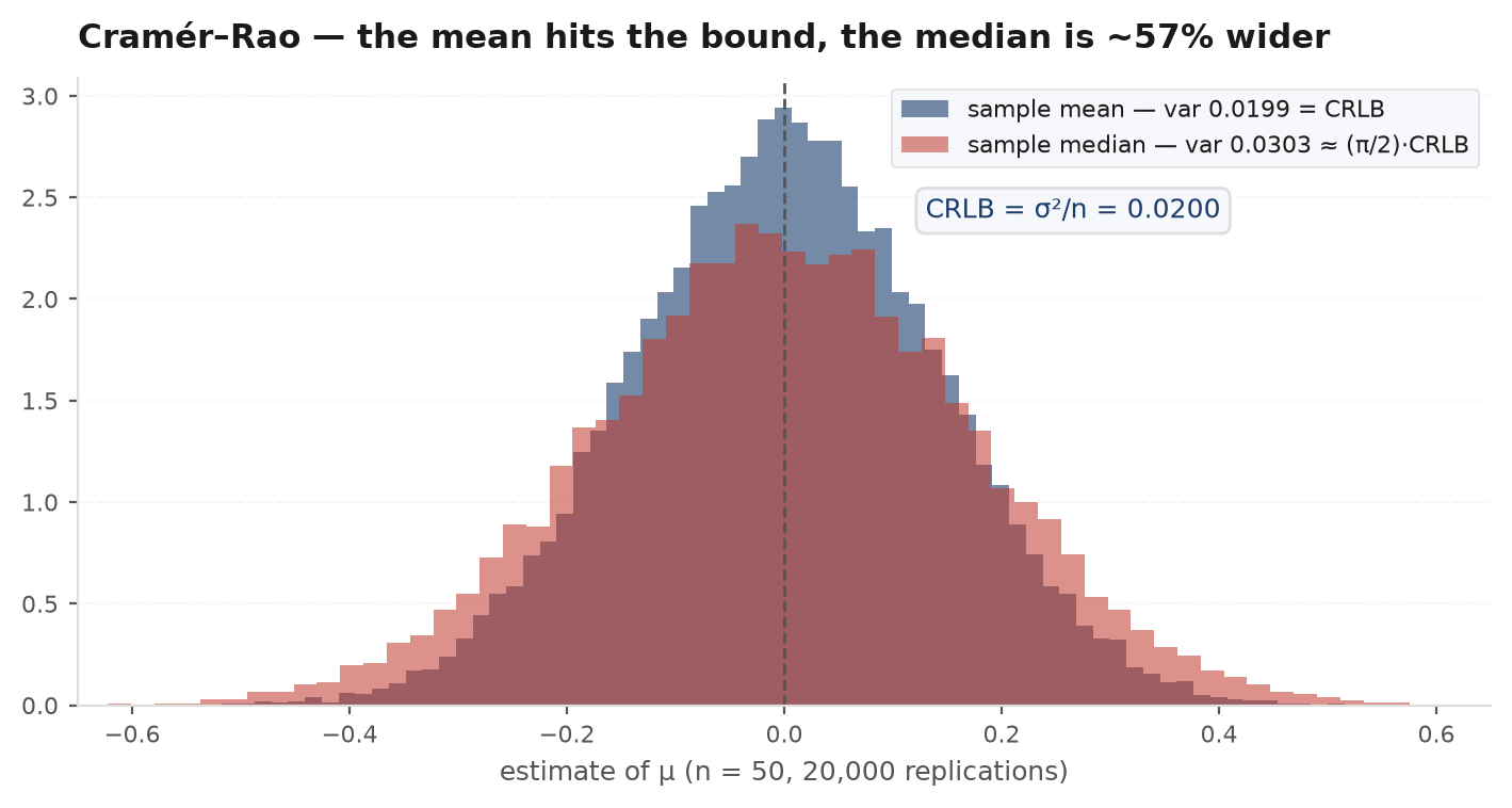
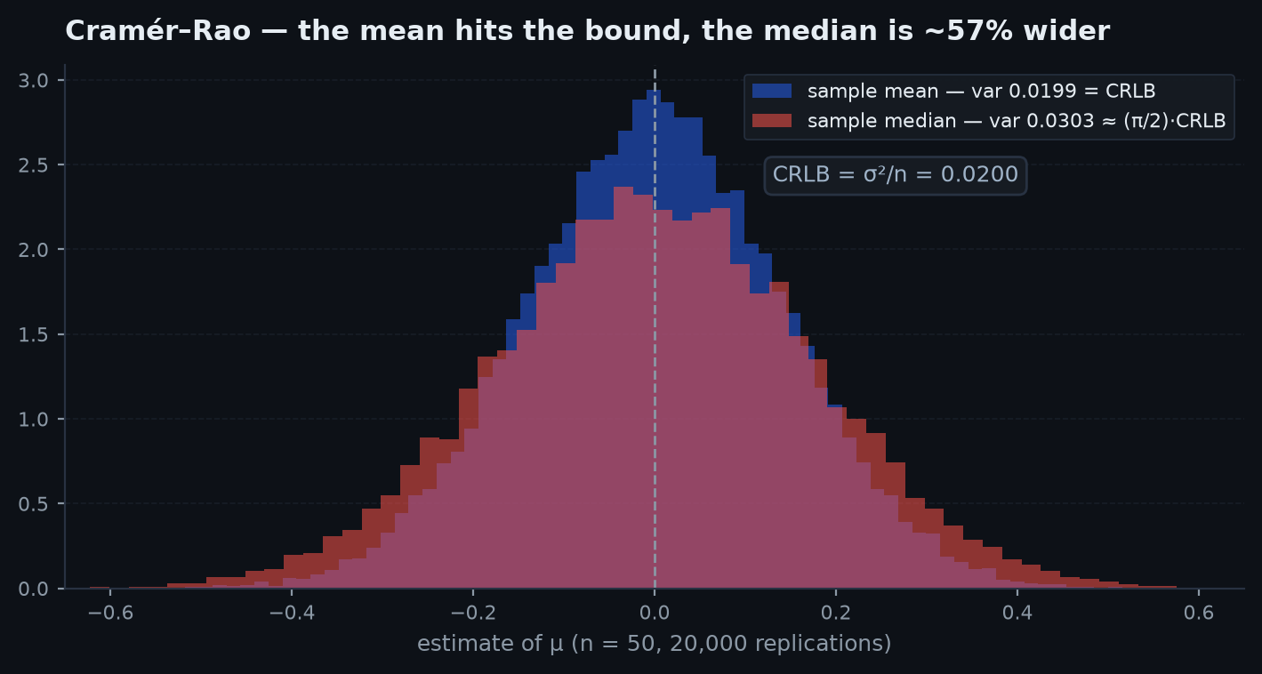
Worked example (Bernoulli). For $f (x; p) = p^{x} (1 - p)^{1 - x}$ , $ln f = x ln p + (1 - x) ln (1 - p)$ , so $U = x / p - (1 - x) / (1 - p)$ and $I (p) = E [U^{2}] = \frac{1}{p ( 1 - p )}$ . The bound is $p (1 - p) / n$ — exactly the variance of $p^= X ˉ$ , which is therefore efficient. For the normal mean, $I (μ) = 1/ σ^{2}$ and $X ˉ$ attains $σ^{2} / n$ : efficient again. With $n = 100, p = 0.5$ the floor is a standard error of $0.25/100 = 0.05$ — no cleverness beats it.

Variance of estimators of a Bernoulli p versus sample size, with the Cramer-Rao lower bound curve p(1-p)/n and the sample proportion sitting on it — The Cramér–Rao bound is a floor under all unbiased estimators. The sample proportion sits exactly on the p(1-p)/n curve — it is efficient; anything above the curve wastes data, anything below is impossible (or biased).

Sufficiency — compressing without losing#

A statistic $T$ is sufficient for $θ$ if the conditional distribution of the data given $T$ does not depend on $θ$ — everything the sample says about $θ$ is already in $T$ . The workable criterion is the factorisation theorem (Fisher–Neyman): $T$ is sufficient iff the likelihood splits as

f (x_{1}, \dots, x_{n}; θ) = g (T (x); θ) h (x) .

Bernoulli / Poisson: $T = \sum X_{i}$ — the likelihood depends on the data only through the count. The order of heads and tails carries no information about $p$ .
Normal: $(X ˉ, s^{2})$ is jointly sufficient for $(μ, σ^{2})$ : two numbers summarise any sample size.
Uniform $[0, θ]$ : $T = max_{i} X_{i}$ , since $f = θ^{- n} 1 {max x_{i} \leq θ}$ — the maximum is the whole story (see order statistics).

Rao–Blackwell makes sufficiency operational: replacing any unbiased estimator $θ^$ by $E [θ^∣ T]$ preserves unbiasedness (tower property) and never increases variance (law of total variance, both proved in joint distributions) — so optimal estimators are always functions of sufficient statistics. And a teaser for what lies beyond: for three or more normal means, the James–Stein estimator shrinks every coordinate toward a common point and beats the sample means in total MSE everywhere — unbiasedness is not just non-sacred, it is dominated. The Bayesian view that makes shrinkage natural is in Bayesian inference.

→Quant lens — every performance number is an estimator

A backtest Sharpe is $S R = r ˉ / s$ — a ratio of two noisy estimators. Propagating their sampling error (delta method, LLN & CLT) gives $se (S R) \approx (1 + S R^{2} /2) / T$ : a strategy with a true annual Sharpe of 1 measured over one year has a standard error near 1 — the estimate is mostly noise. This is why desks (a) demand long samples before believing a Sharpe, (b) shrink estimated alphas and betas toward priors exactly as Rao–Blackwell and James–Stein suggest, and (c) treat a single backtest statistic the way this chapter treats any estimator: as one draw from a wide sampling distribution. The testing machinery built on this view is the gauntlet.

Simulation — checking the theory#

The claims above are all checkable in a few lines: unbiasedness of $s^{2}$ , the MSE ranking of the three divisors, and Jensen’s bias in $s$ .

estimator_check.py

import numpy as np

rng = np.random.default_rng(11)
sigma2, n, reps = 4.0, 10, 200_000
x = rng.normal(0.0, np.sqrt(sigma2), size=(reps, n))

ss = np.sum((x - x.mean(axis=1, keepdims=True)) ** 2, axis=1)
for name, div in [("1/(n-1) unbiased", n - 1), ("1/n     MLE     ", n), ("1/(n+1) min-MSE ", n + 1)]:
    est = ss / div
    print(f"{name}: mean={est.mean():.3f}  bias={est.mean() - sigma2:+.3f}  "
          f"MSE={np.mean((est - sigma2) ** 2):.3f}")
# theory: MSE = 3.556 (n-1), 3.040 (n), 2.909 (n+1)  ->  most biased wins

s = np.sqrt(ss / (n - 1))
print(f"E[s] = {s.mean():.4f} < sigma = {np.sqrt(sigma2):.1f}   (Jensen)")

Practice problems#

→Problem 1 — The three divisors

For normal data, compare the MSE of $S_{c} = c \sum_{i} (X_{i} - X ˉ)^{2}$ as an estimator of $σ^{2}$ for $c = \frac{1}{n - 1}, \frac{1}{n}, \frac{1}{n + 1}$ , and find the optimal $c$ .

Solution. Let $W = \sum (X_{i} - X ˉ)^{2} \sim σ^{2} χ_{n - 1}^{2}$ , so $E [W] = (n - 1) σ^{2}$ and $Var (W) = 2 (n - 1) σ^{4}$ . Then

MSE (c W) = c^{2} 2 (n - 1) σ^{4} + (c (n - 1) - 1)^{2} σ^{4} .

Minimising the quadratic in $c$ gives $c^{⋆} = \frac{n - 1}{2 ( n - 1 ) + ( n - 1 ) ^{2}} = \frac{1}{n + 1}$ . Plugging in: $MSE = \frac{2}{n - 1} σ^{4}$ for the unbiased choice, $\frac{2 n - 1}{n ^{2}} σ^{4}$ for the MLE, and $\frac{2}{n + 1} σ^{4}$ for the optimum. The lesson: unbiasedness costs MSE, and you should know why each divisor exists.

→Problem 2 — German tank

You observe serial numbers of $n$ captured tanks, uniform without replacement from ${1, \dots, N}$ , with maximum $m$ . Estimate $N$ .

Solution. The maximum is sufficient, and by symmetry the $n$ observed tanks split ${1, \dots, N}$ into $n + 1$ exchangeable gaps, so the expected gap above the maximum is $(N - n) / (n + 1)$ : $E [m] = N - \frac{N - n}{n + 1}$ . Solving for $N$ gives the unbiased (indeed UMVU, being a function of the complete sufficient statistic)

N^= m (1 + \frac{1}{n}) - 1 = m + \frac{m}{n} - 1.

Intuition: add the average observed gap on top of the maximum. Numeric: $n = 5$ , $m = 60$ gives $N^= 60 \cdot \frac{6}{5} - 1 = 71$ . The Allies used this on tank gearbox serials; it beat intelligence estimates badly.

→Problem 3 — Efficiency of the sample proportion

You see $k$ heads in $n$ tosses. Show $p^= k / n$ is unbiased and efficient.

Solution. $E [p^] = n p / n = p$ : unbiased. $Var (p^) = p (1 - p) / n$ . From the worked example above, $I (p) = 1/ (p (1 - p))$ , so the Cramér–Rao bound is $p (1 - p) / n$ — attained exactly, so no unbiased estimator does better at any $n$ . The slick close: the Bernoulli score is linear in $x ˉ$ , which is precisely the equality condition in the Cauchy–Schwarz step of the CR proof.

→Problem 4 — Bias-correcting the uniform maximum

From $X_{1}, \dots, X_{n}$ iid Uniform $[0, θ]$ , the natural estimator is $M = max_{i} X_{i}$ . Find its bias and fix it.

Solution. $P (M \leq t) = (t / θ)^{n}$ , so the density is $n t^{n - 1} / θ^{n}$ and $E [M] = \frac{n}{n + 1} θ$ — biased low, because the maximum can never exceed $θ$ . The corrected estimator $θ^= \frac{n + 1}{n} M$ is unbiased with variance $θ^{2} / (n (n + 2))$ — shrinking like $1/ n^{2}$ , dramatically faster than the $1/ n$ of moment-based estimators. Non-regular models can beat the Cramér–Rao rate; the bound’s smoothness assumptions fail here (the support depends on $θ$ ). Full story in maximum likelihood.

→Problem 5 — Mean versus median

For normal data, both the sample mean and sample median estimate $μ$ consistently. Which is better, and by how much?

Solution. The sample median is asymptotically $N (μ, \frac{1}{4 f ( μ ) ^{2} n})$ where $f$ is the density; for the normal, $f (μ) = 1/ (σ 2 π)$ , giving variance $\frac{π}{2} \cdot \frac{σ ^{2}}{n} \approx 1.57 σ^{2} / n$ versus $σ^{2} / n$ for the mean: the median is only $2/ π \approx 64%$ efficient — you throw away a third of your data by using it. The twist worth knowing: under fat tails the ranking flips (for the Cauchy the mean does not even converge — see when the CLT fails), which is why robust statistics exist and why the “right” estimator depends on the tail model.

Next: a systematic machine for generating good estimators — maximise the likelihood — and when that machine breaks. Maximum likelihood & method of moments.