Bootstrap & resampling

Most statistics you care about — the median, a Sharpe ratio, a maximum drawdown — have no clean formula for their sampling distribution. The bootstrap’s answer is radical: treat the sample as if it were the population and simulate the sampling distribution by resampling. This chapter builds the plug-in principle, the nonparametric and parametric bootstrap, the jackknife, and permutation tests — proves the pieces that can be proved — and then shows, honestly, the famous cases where the bootstrap fails: the maximum, heavy tails, and dependent data.

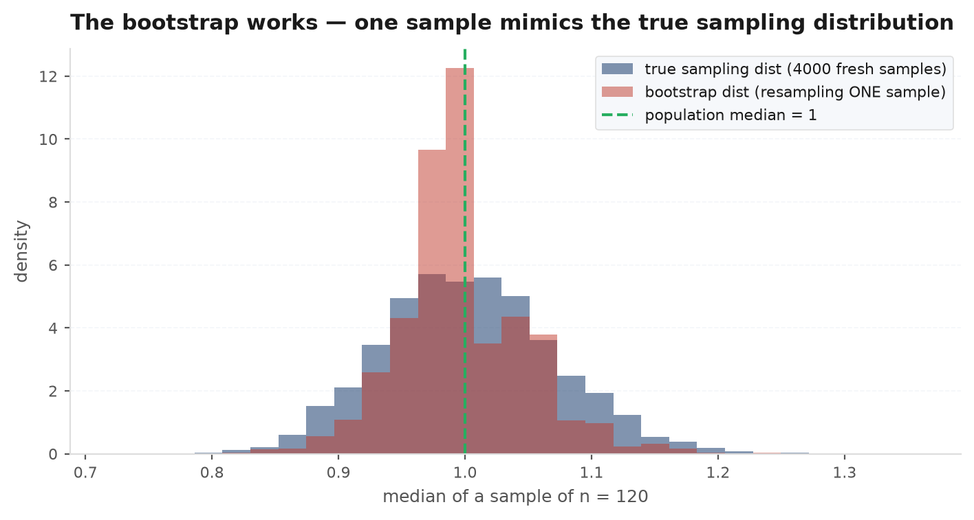
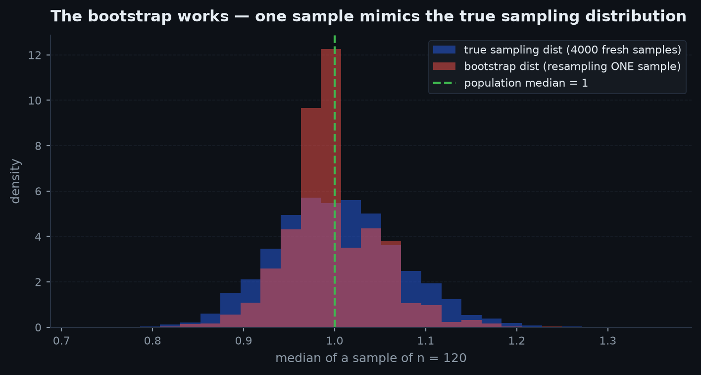
✦Intuition — the world in a grain of sand

You want to know how much your statistic would wobble if you could rerun history. You cannot rerun history — but your sample of $n$ observations is itself an estimate of the distribution history draws from. So rerun that: draw $n$ points from your own data with replacement, recompute the statistic, repeat thousands of times. The spread of those recomputed values estimates the spread you actually care about. Two approximations are being made — the empirical distribution stands in for the true one, and Monte Carlo stands in for exhaustive enumeration — and the whole theory of the bootstrap is about when the first approximation is good enough.

The plug-in principle and the empirical CDF#

Write the parameter of interest as a functional of the distribution: $θ = T (F)$ — the mean is $T (F) = \int x d F (x)$ , the median is $F^{- 1} (1/2)$ , a Sharpe ratio is a ratio of two such functionals. The empirical CDF of a sample $X_{1}, \dots, X_{n}$ is

F_{n} (x) = \frac{1}{n} i = 1 \sum n 1 {X_{i} \leq x},

the distribution putting mass $1/ n$ on each observed point. The plug-in principle estimates $θ$ by $θ = T (F_{n})$ . Why should this work? Because the empirical CDF converges to the truth, uniformly:

✦Theorem (Glivenko–Cantelli) — statement

For iid $X_{1}, X_{2}, \dots \sim F$ ,

x \in R sup F_{n} (x) - F (x) a.s. 0.

Pointwise convergence at each $x$ is just the strong law of large numbers applied to the indicators $1 {X_{i} \leq x}$ (see LLN & the CLT); the content of Glivenko–Cantelli is that the convergence is uniform over all $x$ simultaneously — proved by controlling the CDF on a finite grid of quantiles and using monotonicity to squeeze everything in between. Uniform closeness of $F_{n}$ to $F$ is what licenses substituting one for the other inside any reasonably smooth functional $T$ .

The nonparametric bootstrap#

The sampling distribution of $θ$ is determined by $F$ (unknown) and $n$ . The bootstrap replaces $F$ by $F_{n}$ , under which sampling $n$ iid points means drawing $n$ times with replacement from the observed data. The algorithm:

For $b = 1, \dots, B$ : draw a resample $X_{1}^{*}, \dots, X_{n}^{*}$ with replacement from the data; compute $θ_{b}^{*} = T (resample)$ .
Use the empirical distribution of ${θ_{b}^{*}}$ as the estimated sampling distribution: its standard deviation is the bootstrap standard error, its quantiles feed confidence intervals.

✦Proof sketch — why the bootstrap works (and what it needs)

The object of interest is the law of the (centred, scaled) statistic, $G_{n} (F) = L (n (θ - θ (F)))$ . The bootstrap estimates it by $G_{n} (F_{n})$ — same map, plugged-in argument. Consistency needs three ingredients: (1) $F_{n} \to F$ (Glivenko–Cantelli); (2) the map $F \mapsto G_{n} (F)$ is continuous in the right topology — the statistic depends smoothly on the distribution (Hadamard differentiability of $T$ ); (3) the limit law is continuous in $F$ . For the mean, everything is explicit: conditional on the data, the resample mean has expectation $X ˉ$ and variance $σ^{2} / n$ (plug-in variance), and the CLT applies to the resampling too — so the bootstrap distribution converges to the same normal limit as the true sampling distribution. Every classical bootstrap failure below is a failure of ingredient (2): the statistic is not a smooth functional of $F$ at the point that matters.

Worked example (fully by hand). Data: ${1, 3, 5}$ , statistic = mean, so $θ = 3$ . With $n = 3$ there are only $3^{3} = 27$ equally likely resamples, so we can compute the exact bootstrap distribution, no Monte Carlo needed. Conditional on the data, each draw $X^{*}$ has mean 3 and variance

Var (X^{*}) = \frac{1}{3} [(1 - 3)^{2} + (3 - 3)^{2} + (5 - 3)^{2}] = \frac{8}{3},

the plug-in variance (divide by $n$ , not $n - 1$ — the bootstrap world’s population is the sample). The bootstrap variance of the resample mean is therefore $Var (X ˉ^{*}) = \frac{8/3}{3} = \frac{8}{9}$ , giving bootstrap standard error $8 /3 \approx 0.943$ . Compare the textbook $s / n = 2/ 3 \approx 1.155$ : the bootstrap se is smaller by the factor $(n - 1) / n$ — a known small-sample bias of the plug-in variance that vanishes as $n$ grows.

Histogram of bootstrap replicates of a statistic with the observed value and percentile interval marked — A bootstrap distribution: thousands of recomputed statistics, one per resample. Its standard deviation estimates the standard error; its quantiles give the percentile interval. The shape — skew, lumpiness — is information a formula-based se throws away.

Confidence intervals: percentile, basic, bootstrap-t#

Let $q_{α}^{*}$ denote the $α$ -quantile of the bootstrap replicates. Three standard 90% intervals:

Interval	Formula	Logic
Percentile	[q₀.₀₅, q₀.₉₅]	Read the bootstrap distribution directly
Basic (pivotal)	[2θ̂ − q₀.₉₅, 2θ̂ − q₀.₀₅]	Bootstrap the error θ̂* − θ̂, flip it around θ̂
Bootstrap-t	[θ̂ − t₀.₉₅·se, θ̂ − t₀.₀₅·se]	Bootstrap the studentised statistic (θ̂* − θ̂)/se*

The percentile interval assumes the bootstrap distribution sits around $θ$ the way the sampling distribution sits around $θ$ — true only if the distribution of $θ - θ$ is symmetric and unbiased. The basic interval fixes the direction of the flip (if $θ$ tends to overshoot, the interval should extend further below). The bootstrap-t studentises first, which typically gives the most accurate coverage (second-order accurate, $O (1/ n)$ coverage error versus $O (1/ n)$ for percentile) at the cost of needing a standard-error estimate inside every resample. The parametric bootstrap is the same machinery with a fitted model in place of $F_{n}$ : fit $F_{ψ}$ (say a normal or a fitted MLE model), simulate samples of size $n$ from it, recompute. It is more efficient when the model is right and biased when it is wrong — the usual trade.

The jackknife#

The bootstrap’s deterministic grandparent: recompute the statistic $n$ times, leaving out one observation each time. Write $θ_{(i)}$ for the leave-one-out estimate and $θ ˉ_{(\cdot)}$ for their average. The jackknife estimates

bias_{jack} = (n - 1) (θ ˉ_{(\cdot)} - θ), se_{jack}^{2} = \frac{n - 1}{n} i = 1 \sum n (θ_{(i)} - θ ˉ_{(\cdot)})^{2} .

✦Derivation — the jackknife bias estimate, and the sanity check on the mean

Suppose the estimator’s bias expands as $E [θ_{n}] = θ + a / n + O (1/ n^{2})$ . The leave-one-out estimates use $n - 1$ points, so $E [θ ˉ_{(\cdot)}] = θ + a / (n - 1) + O (1/ n^{2})$ . Then

(n - 1) (E [θ ˉ_{(\cdot)}] - E [θ_{n}]) = (n - 1) a (\frac{1}{n - 1} - \frac{1}{n}) + O (1/ n) = \frac{a}{n} + O (1/ n),

which matches the leading bias term — so subtracting it kills the $O (1/ n)$ bias. Sanity check on the mean: for $θ = X ˉ$ , each $θ_{(i)} = \frac{n X ˉ - X _{i}}{n - 1}$ , whose average over $i$ is $\frac{n X ˉ - X ˉ}{n - 1} = X ˉ$ . So $θ ˉ_{(\cdot)} = θ$ and the estimated bias is exactly zero — as it must be, since the sample mean is unbiased. Meanwhile the jackknife variance formula reproduces $s^{2} / n$ exactly for the mean (a two-line algebra check), which is why the odd-looking factor $(n - 1) / n$ is there. The jackknife fails for non-smooth statistics like the median — its leave-one-out perturbations are too small to explore the distribution — which is precisely where the bootstrap takes over.

Permutation tests#

Resampling also yields exact hypothesis tests. Two samples, $X_{1}, \dots, X_{m}$ and $Y_{1}, \dots, Y_{k}$ ; null hypothesis: the two groups have the same distribution. Under that null the group labels are arbitrary — the combined data are exchangeable — so every one of the $(m m + k)$ relabellings was equally likely to have produced the observed split.

✦Proof — exactness of the permutation test

Let $S$ be any test statistic (say the difference in group means) and let $S_{(1)}, \dots, S_{(K)}$ be its values over all $K = (m m + k)$ label assignments. Under $H_{0}$ , conditional on the pooled data, the observed assignment is uniform over the $K$ possibilities — that is exchangeability. Hence the permutation p-value $p = \frac{1}{K} # {j : S_{(j)} \geq S_{obs}}$ satisfies $P (p \leq α ∣ H_{0}) \leq α$ for every $n$ — no asymptotics, no normality, no variance formula. The test is exact for any statistic you like; the choice of statistic affects only power. In practice you sample a few thousand random permutations instead of enumerating all $K$ , adding only Monte-Carlo error you control.

Worked example. Strategy returns on 4 days ${2, 3, 1, 4}$ (mean 2.5), benchmark on 3 days ${- 1, 0, 1}$ (mean 0). Observed difference 2.5. There are $(4 7) = 35$ relabellings. Writing $S_{4}$ for the sum of the 4-group, the difference is $(7 S_{4} - 40) /12 \geq 2.5 ⟺ S_{4} \geq 10$ — achieved only by taking the four largest values ${4, 3, 2, 1}$ , and since the pool contains two tied 1s there are exactly two such splits, so $p = 2/35 \approx 0.057$ . With seven data points the test has done everything the data permit — and the granularity (smallest possible p-value $1/35$ ) is itself a lesson about tiny samples.

When the bootstrap fails#

The bootstrap is not magic; it inherits the smoothness assumptions in the proof sketch above. Three canonical failures, in increasing order of practical importance for quants:

1. Extremes — the maximum. Take $X_{i} \sim Uniform (0, θ)$ and $θ = X_{(n)} = max_{i} X_{i}$ . The true sampling theory (from Order statistics) says $n (θ - X_{(n)}) / θ$ converges to an Exponential(1) — a smooth, atomless limit. The bootstrap version cannot reproduce it:

P (X_{(n)}^{*} = X_{(n)}) = 1 - (1 - \frac{1}{n})^{n} ⟶ 1 - e^{- 1} \approx 0.632,

because the resample max equals the sample max whenever at least one draw hits the largest observation. So the bootstrap distribution of $n (θ - θ^{*})$ has a permanent atom of mass 0.632 at zero — it converges to the wrong limit, no matter how large $n$ or $B$ . The failure is ingredient (2): the max is not a smooth functional of $F$ . (Remedies exist — the $m$ -out-of- $n$ bootstrap with $m / n \to 0$ , or parametric extreme-value theory.)

bootstrap_max_fails.py

import numpy as np

rng = np.random.default_rng(11)
n, B, theta = 100, 4000, 1.0

x = rng.uniform(0, theta, n)
mx = x.max()

# bootstrap the maximum
boot_max = np.array([rng.choice(x, n, replace=True).max() for _ in range(B)])
atom = (boot_max == mx).mean()
print(f"P*(max* == max)      : {atom:.3f}   (theory: 1 - (1-1/n)^n -> 0.632)")

# compare: true sampling dist of n*(theta - max)/theta is ~ Exp(1), atomless.
# the bootstrap analogue n*(max - max*)/max has a big atom at exactly 0:
print(f"bootstrap mass at 0  : {(mx - boot_max == 0).mean():.3f}")
# ~0.63 of all bootstrap replicates sit on a single point -- the bootstrap
# 'distribution' of the max is degenerate and its CIs are garbage.

2. Heavy tails. If $Var (X) = \infty$ (a Pareto with tail index below 2, a t(2) — see the distribution zoo), the sample mean has a non-normal stable limit, and the bootstrap distribution of the mean fails to converge to it: each resample is dominated by whether the few enormous observations were drawn 0, 1, or 3 times, so the bootstrap distribution stays random even as $n \to \infty$ . For drawdown and tail-risk work on fat-tailed returns, bootstrap results deserve wide error bars of their own.

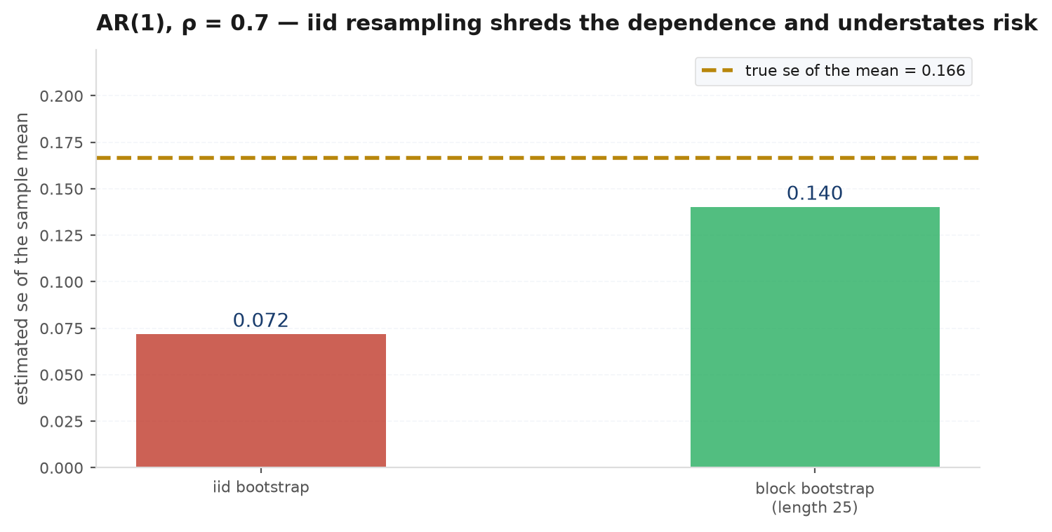
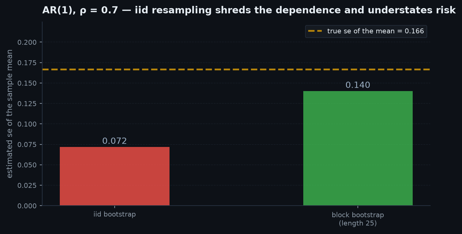
3. Dependence — and the block bootstrap. The iid bootstrap destroys time structure: resampling daily returns one at a time scrambles autocorrelation and volatility clustering, so it understates the variance of anything that accumulates. From time-series statistics, positive autocorrelation inflates the variance of the sample mean by the factor $1 + 2 \sum_{k} ρ_{k}$ — the iid bootstrap silently sets that factor to 1. The block bootstrap fixes it by resampling contiguous blocks (length $ℓ$ ) instead of single points, preserving dependence within blocks and sacrificing only the joints between them.

Comparison of iid resampling versus block resampling of an autocorrelated series, with the block version preserving runs — IID resampling (top) shreds an autocorrelated series into white noise; block resampling (bottom) keeps runs of consecutive days intact, so clustering and momentum survive into the resamples. Block length trades bias (too short: dependence broken) against variance (too long: too few distinct blocks).

iid_vs_block.py

import numpy as np

rng = np.random.default_rng(11)
n, phi = 2000, 0.5                       # AR(1) daily returns, rho_1 = 0.5
eps = rng.normal(0, 0.01, n)
r = np.empty(n); r[0] = eps[0]
for t in range(1, n):
    r[t] = phi * r[t-1] + eps[t]

true_factor = (1 + phi) / (1 - phi)      # variance inflation for the mean = 3.0
se_true = r.std(ddof=1)/np.sqrt(n) * np.sqrt(true_factor)

B, ell = 2000, 25
iid  = np.array([rng.choice(r, n, replace=True).mean() for _ in range(B)])
nblk = n // ell
starts = rng.integers(0, n - ell + 1, size=(B, nblk))
blocks = r[starts[:, :, None] + np.arange(ell)]      # (B, nblk, ell)
blk  = blocks.reshape(B, -1).mean(axis=1)

print(f"true se of mean : {se_true:.5f}")
print(f"iid bootstrap   : {iid.std():.5f}   (too small by ~sqrt(3))")
print(f"block bootstrap : {blk.std():.5f}   (close to the truth)")

→Quant lens — honest drawdown distributions via block bootstrap

This is exactly why edgekit’s forward-risk engine resamples blocks of daily returns: ek.validation.block_bootstrap_mc(returns, block=5, horizon=252) stitches 5-day blocks into thousands of synthetic years and returns the terminal-wealth and max-drawdown distributions, and ek.validation.dd95 reads off the 95th-percentile drawdown to size against. Single-day resampling would break the volatility clustering that makes real drawdowns deep — losses beget losses — and would report a reassuringly, wrongly thin drawdown tail. The single realised historical drawdown is one draw from this distribution; sizing to it is survivorship bias applied to your own history. See Monte Carlo & risk for the applied treatment.

Practice problems#

→Problem 1 — Bootstrap standard error of the median

You have 101 daily P&L observations and want a standard error for the median. Explain why the textbook route is awkward, give the bootstrap recipe, and state one caveat.

Solution. The asymptotic variance of the sample median is $1/ (4 n f (m)^{2})$ where $f (m)$ is the density at the true median — it requires density estimation, which is noisy and bandwidth-dependent; and the jackknife is inconsistent for the median (non-smooth statistic). The bootstrap: resample the 101 points with replacement $B \approx 2000$ times, take the median of each resample, report the standard deviation of the $B$ medians. It is consistent because the median is Hadamard-differentiable wherever $f (m) > 0$ . Caveat: the bootstrap distribution of a median is discrete (it can only take observed values), so for small $n$ it is lumpy — quantile-based intervals can behave better than the raw se, and smoothing the bootstrap slightly improves accuracy.

→Problem 2 — Why can the percentile interval undercover?

A colleague reports a 90% percentile-bootstrap CI for a strategy’s Sharpe ratio from two years of data. Give two distinct reasons the true coverage may be below 90%.

Solution. (1) Bias and skew. The percentile interval implicitly assumes $θ^{*} - θ$ has the same distribution as $θ - θ$ and that this distribution is symmetric. A Sharpe estimator on two years is skewed (its denominator is random) and biased; the percentile interval reads the skew in the wrong direction — the basic interval flips it, and bootstrap-t or BCa corrects it properly. Coverage error is $O (1/ n)$ for percentile vs $O (1/ n)$ for studentised methods. (2) Dependence. Daily returns are autocorrelated and volatility-clustered; the iid bootstrap under-disperses the resampled Sharpes (variance-inflation factor silently set to 1), shrinking the interval. The fix is the block bootstrap — and even then, two years is little data for a ratio statistic. A complete answer names both failure modes: interval construction error and resampling-scheme error.

→Problem 3 — Design a permutation test: strategy vs benchmark

Given 252 paired daily returns (strategy, benchmark), design an exact test of “no outperformance” without distributional assumptions.

Solution. Work with paired differences $d_{t} = r_{t}^{strat} - r_{t}^{bench}$ . The sharp null is that the strategy and benchmark are exchangeable within each day, i.e. each $d_{t}$ is symmetric about 0 — under it, flipping the sign of any $d_{t}$ leaves the joint distribution unchanged. So: compute $S_{obs} = d ˉ$ ; for each of $B = 10, 000$ iterations draw random signs $ε_{t} \in {\pm 1}$ and recompute $d ˉ^{(b)} = \frac{1}{252} \sum ε_{t} d_{t}$ ; p-value = fraction of $d ˉ^{(b)} \geq S_{obs}$ . Pairing by day kills the shared market factor (the dominant variance), a two-sample label shuffle would not — that is the design point being tested. Caveats to volunteer: sign-flipping assumes symmetry of $d_{t}$ under the null and independence across days; with autocorrelation, flip signs of blocks of days instead, trading a little exactness for honesty.

→Problem 4 — Show that the bootstrap fails for the maximum

Let $X_{1}, \dots, X_{n}$ be iid Uniform(0, θ). Show the nonparametric bootstrap is inconsistent for the distribution of the maximum.

Solution. Truth first: $P (n (θ - X_{(n)}) / θ > t) = P (X_{(n)} < θ (1 - t / n)) = (1 - t / n)^{n} \to e^{- t}$ — an Exponential(1) limit, continuous with no mass at 0. Bootstrap: conditional on the data, each resample draw misses the sample maximum with probability $1 - 1/ n$ , so

P^{*} (X_{(n)}^{*} = X_{(n)}) = 1 - (1 - 1/ n)^{n} \to 1 - e^{- 1} \approx 0.632.

Hence the bootstrap law of $n (X_{(n)} - X_{(n)}^{*})$ places asymptotic mass 0.632 at exactly 0, while the true limit places mass 0 there — the bootstrap distribution does not converge to the truth, for any sample size. One line of intuition to close: the max depends on a single order statistic, and resampling from $n$ atoms cannot generate new candidate maxima above it. Fixes: $m$ -out-of- $n$ bootstrap ( $m \to \infty, m / n \to 0$ ), or a parametric/EVT model for the tail.

→Problem 5 — Exact bootstrap, no computer

For data ${0, 6}$ (n = 2) and the statistic $X ˉ$ , write down the exact bootstrap distribution of $X ˉ^{*}$ and its standard error.

Solution. Four equally likely resamples: $(0, 0), (0, 6), (6, 0), (6, 6)$ , giving $X ˉ^{*} \in {0, 3, 3, 6}$ — the distribution puts mass $1/4, 1/2, 1/4$ on $0, 3, 6$ . Mean 3 (= $X ˉ$ , as always); variance $\frac{1}{4} (9) + \frac{1}{2} (0) + \frac{1}{4} (9) = 4.5$ , so bootstrap se $\approx 2.12$ . Check against theory: plug-in variance $σ^{2} = \frac{1}{2} (9 + 9) = 9$ , and $σ^{2} / n = 4.5$ ✓. This tiny example is worth carrying with you: it shows the bootstrap is a deterministic object (Monte Carlo only approximates it) and that its centre is $θ$ , not $θ$ — the whole reason basic/t intervals recentre.

Next: the block bootstrap existed because financial data are dependent in time — now meet that dependence head-on: stationarity, autocorrelation, AR(1), and why regressions on trending series lie. Time-series statistics.