Simulation & Monte Carlo

When an expectation has no closed form — a path-dependent option, a drawdown distribution, a posterior — you estimate it by sampling. Monte Carlo turns every integral into an average, and the entire subject reduces to two questions: how do I draw from the distribution I need? and how do I shrink the variance of the average? This chapter derives the estimator and its $1/ n$ error law, builds the classic sampling algorithms (inverse transform, acceptance–rejection, Box–Muller, Cholesky), and ends with importance sampling — the tool that makes rare-event probabilities computable.

✦Intuition — integration by gambling

Any expectation is an integral, and any integral over a probability density is an expectation. If you can draw samples $X_{1}, \dots, X_{n}$ from the density, the law of large numbers (chapter 7) guarantees the sample average of $g (X_{i})$ converges to $E [g (X)]$ , and the CLT tells you exactly how fast. The magic is what the error rate does not depend on: the dimension of the integral. A 100-dimensional basket-option price converges at the same $1/ n$ rate as a one-dimensional one — which is why Monte Carlo owns high-dimensional finance while quadrature grids die of the curse of dimensionality.

The Monte Carlo estimator and its error#

Suppose you want $θ = E [g (X)]$ and can simulate iid copies of $X$ . The Monte Carlo estimator is the plain average

θ^_{n} = \frac{1}{n} i = 1 \sum n g (X_{i}), E [θ^_{n}] = θ (unbiased) .

✦Proof — the standard error and the 1/√n law

By independence, variances add: $Var (θ^_{n}) = \frac{1}{n ^{2}} \sum_{i} Var (g (X_{i})) = σ_{g}^{2} / n$ where $σ_{g}^{2} = Var (g (X))$ . So the root-mean-square error is

se (θ^_{n}) = \frac{σ _{g}}{n},

and by the CLT, $θ^_{n} \approx N (θ, σ_{g}^{2} / n)$ for large $n$ , giving the reportable interval $θ^_{n} \pm 1.96 σ^_{g} / n$ with $σ^_{g}$ the sample standard deviation of the $g (X_{i})$ . Nothing in the derivation mentioned the dimension of $X$ — only the variance of the scalar $g (X)$ matters. The price of the square root: one more decimal digit of accuracy costs $100 \times$ the samples. Every variance-reduction technique below exists to shrink $σ_{g}$ instead of growing $n$ .

Worked example — estimating $π$ . Throw uniform points on the unit square; $g (X) = 1 {x^{2} + y^{2} \leq 1}$ has mean $p = π /4 \approx 0.7854$ , a Bernoulli with variance $p (1 - p) \approx 0.1685$ . The estimator $π^= 4 g ˉ$ therefore has standard error $4 0.1685/ n \approx 1.642/ n$ . With $n = 1 0^{6}$ darts: se $\approx 0.00164$ — you get $π \approx 3.14$ reliably, but the fourth digit is already a coin flip. To pin down $3.14159$ (se $\approx 5 \times 1 0^{- 6}$ ) you would need $n \approx (1.642/5 \times 1 0^{- 6})^{2} \approx 1 0^{11}$ darts. Monte Carlo is a blunt instrument for precision — and a scalpel for dimension.

→Quant lens — the backtest is a Monte Carlo estimate

A backtest average of

n

trade returns is

θ^_{n}

with

g =

P&L per trade — same estimator, same

σ / n

error bar, except the market hands you one sample path and you cannot rerun it. Simulation restores the ability to rerun: resample the trades (bootstrap) or simulate the price process (simulating markets) and the distribution of Sharpe, drawdown, and ruin becomes an ordinary Monte Carlo computation. That is the entire logic of the applied Monte Carlo chapter.

Inverse transform sampling#

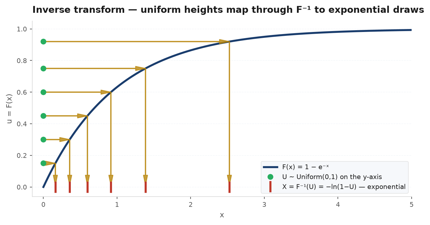
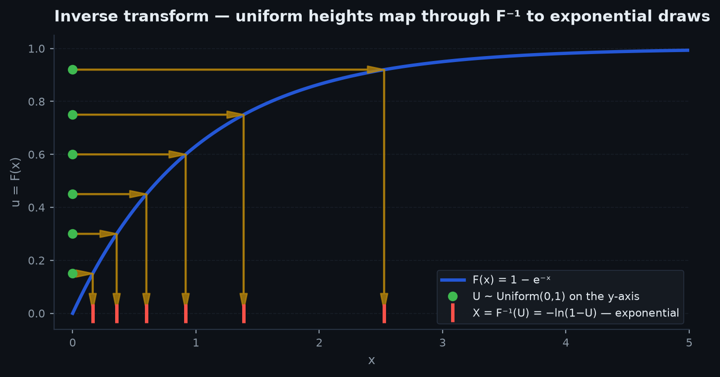
Every sampler starts from uniforms — that is what a random number generator emits. The inverse transform method converts them into any distribution with a computable quantile function: if $U \sim Unif (0, 1)$ and $F$ is a CDF with generalised inverse $F^{- 1} (u) = in f {x : F (x) \geq u}$ , then $X = F^{- 1} (U)$ has CDF $F$ .

✦Proof — via the probability integral transform

For any $x$ , the event ${F^{- 1} (U) \leq x}$ is exactly ${U \leq F (x)}$ : if $u \leq F (x)$ then $x$ is in the set whose infimum defines $F^{- 1} (u)$ , so $F^{- 1} (u) \leq x$ ; conversely $F^{- 1} (u) \leq x$ implies $F (x) \geq u$ by right-continuity and monotonicity of $F$ . Hence

P (X \leq x) = P (U \leq F (x)) = F (x),

since $P (U \leq u) = u$ . This is the same probability integral transform proved in order statistics — there it turned data into uniforms (p-values); here it runs in reverse, turning uniforms into data.

Worked example — exponential. For $F (x) = 1 - e^{- λ x}$ , solve $u = 1 - e^{- λ x}$ to get $x = - ln (1 - u) / λ$ , and since $1 - U \sim U$ , the one-liner is $X = - ln (U) / λ$ . Concretely with $λ = 2$ : $u = 0.30 \Rightarrow x = - ln (0.70) /2 = 0.178$ ; $u = 0.95 \Rightarrow x = - ln (0.05) /2 = 1.498$ . The method also covers discrete distributions (step through cumulative probabilities until they exceed $u$ ) — which is the honest answer to the classic exercise “simulate from an arbitrary CDF.”

A CDF curve with uniform draws on the vertical axis mapped through the inverse CDF to samples on the horizontal axis, next to the resulting histogram matching the target density — Inverse transform sampling: uniform draws on the vertical axis are pushed through the quantile function F^{-1} to the horizontal axis. Dense regions of the target density correspond to steep stretches of F, so equal slices of u land more points there — the histogram of the mapped samples reproduces the target.

Acceptance–rejection#

When $F^{- 1}$ is unavailable but the density $f$ is computable, sample from an easy proposal density $h$ dominating $f$ : choose $M$ with $f (x) \leq M h (x)$ for all $x$ , then repeat: draw $Y \sim h$ and $U \sim Unif (0, 1)$ , and accept $Y$ if $U \leq f (Y) / (M h (Y))$ .

✦Proof sketch — accepted draws have density f, and efficiency is 1/M

The joint chance of proposing near $x$ and accepting is $h (x) d x \cdot \frac{f ( x )}{M h ( x )} = \frac{f ( x )}{M} d x$ . Integrating over $x$ , the overall acceptance probability is $\int f / M = 1/ M$ . By Bayes, the density of $Y$ given acceptance is

\frac{f ( x ) / M}{1/ M} = f (x) .

Exactly the target — and the number of proposals per accepted sample is geometric with mean $M$ . So the whole game is finding a proposal that hugs $f$ tightly: $M$ close to 1 means almost nothing is wasted. Worked numbers: to sample $Beta (2, 2)$ , $f (x) = 6 x (1 - x)$ , from a uniform proposal $h = 1$ : the max of $f$ is $6 \cdot \frac{1}{2} \cdot \frac{1}{2} = 1.5$ , so $M = 1.5$ and you accept $1/1.5 = 66.7%$ of proposals — three draws for every two samples. In high dimensions $M$ typically blows up exponentially, which is why rejection is a low-dimensional tool.

Box–Muller and Cholesky: manufacturing normals#

The normal CDF has no closed-form inverse, so normals get their own trick. Box–Muller: from two independent uniforms $U_{1}, U_{2}$ ,

Z_{1} = - 2 ln U_{1} cos (2 π U_{2}), Z_{2} = - 2 ln U_{1} sin (2 π U_{2})

are independent standard normals.

✦Proof sketch — Box–Muller via polar coordinates

Write a standard normal pair in polar form, $(Z_{1}, Z_{2}) = (R cos Θ, R sin Θ)$ . The joint density $\frac{1}{2 π} e^{- (z_{1}^{2} + z_{2}^{2}) /2}$ is rotationally symmetric, so $Θ \sim Unif (0, 2 π)$ independently of $R$ , and the squared radius satisfies

P (R^{2} > r) = e^{- r /2} ⟹ R^{2} \sim Exponential (1/2),

(the chi-square with 2 df from the distribution zoo). Both ingredients are inverse-transform-easy: $R^{2} = - 2 ln U_{1}$ and $Θ = 2 π U_{2}$ . Substituting back gives the formulas. Note the trap this exposes: to get a uniform point on a circle, take $(cos Θ, sin Θ)$ — but a uniform point in a disk needs $R = U$ , not $R = U$ , because area grows like $r^{2}$ .

Correlated normals via Cholesky. Portfolios need normals with a prescribed covariance $Σ$ . Factor $Σ = L L^{⊤}$ (lower-triangular $L$ , which exists because covariance matrices are PSD — see joint distributions) and set $X = L Z$ for iid standard normals $Z$ . Then $Cov (X) = L E [Z Z^{⊤}] L^{⊤} = L L^{⊤} = Σ$ , and $X$ is normal because linear combinations of normals are normal. In the $2 \times 2$ correlation case the factorisation is worth memorising: solving

(1 ρ ρ 1) = (ℓ_{11} ℓ_{21} 0 ℓ_{22}) (ℓ_{11} 0 ℓ_{21} ℓ_{22}) ⟹ X_{1} = Z_{1}, X_{2} = ρ Z_{1} + 1 - ρ^{2} Z_{2} .

Check it: $Var (X_{2}) = ρ^{2} + (1 - ρ^{2}) = 1$ and $Cov (X_{1}, X_{2}) = ρ$ . With $ρ = 0.6$ : $X_{2} = 0.6 Z_{1} + 0.8 Z_{2}$ — the $3 - 4 - 5$ triangle of correlated simulation. This one line is the seed of every correlated-asset simulator, and the regression-line structure it encodes is exactly the bivariate-normal conditional expectation derived in chapter 5.

Importance sampling: buying variance with bias-free money#

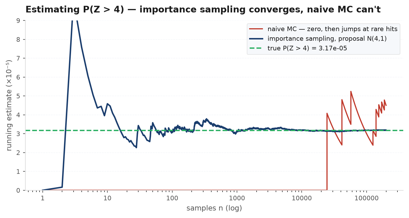
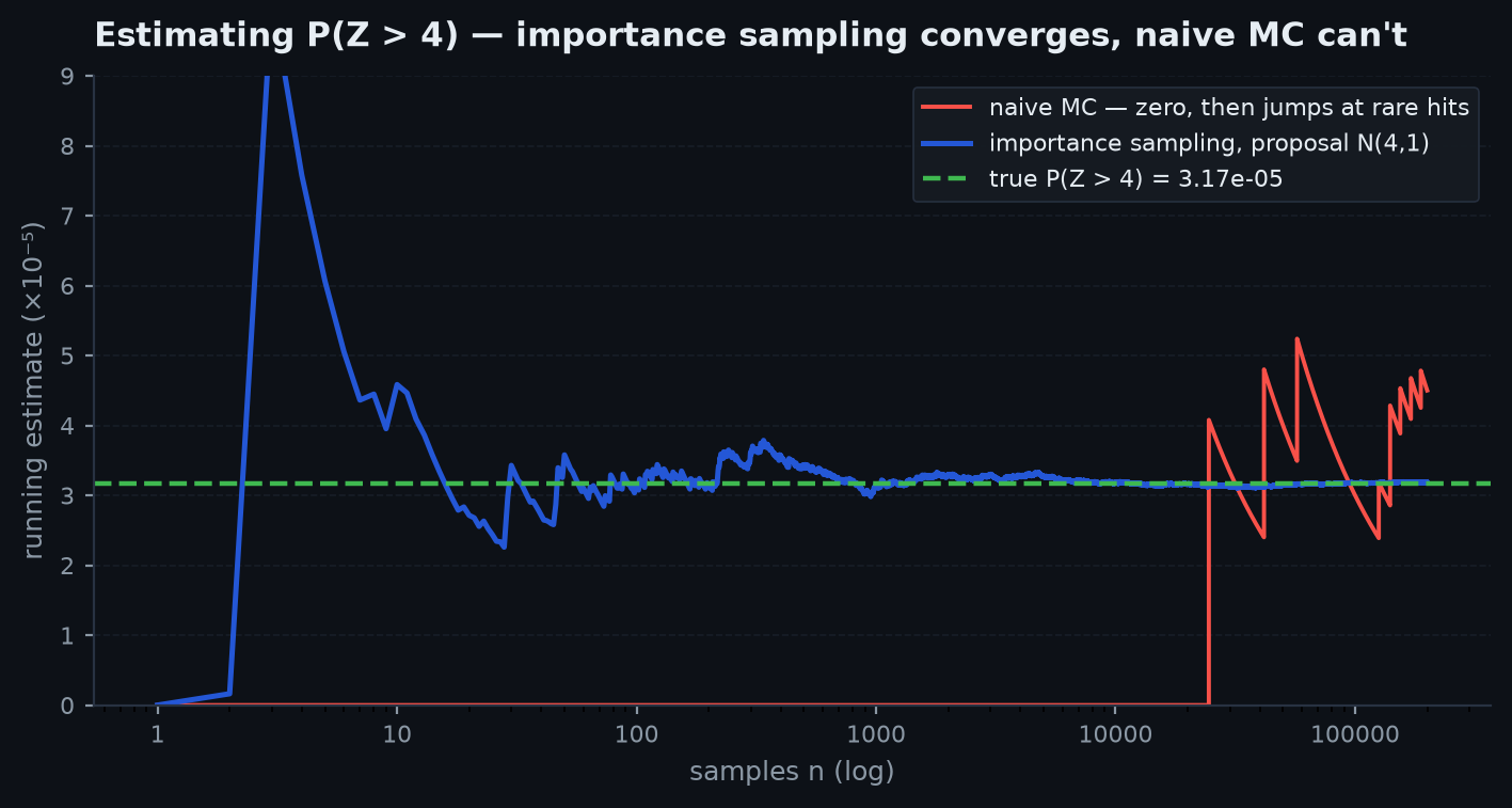
The naive estimator fails exactly where finance cares most: rare events. To estimate $θ = P (Z > 4) \approx 3.17 \times 1 0^{- 5}$ for $Z \sim N (0, 1)$ , naive sampling waits ~31,600 draws per hit. Importance sampling samples where the action is and reweights. For any proposal density $q$ that is positive wherever $f g \neq = 0$ ,

θ = \int g (x) f (x) d x = \int g (x) \frac{f ( x )}{q ( x )} q (x) d x = E_{q} [g (Y) \frac{f ( Y )}{q ( Y )}], Y \sim q,

so the weighted average $θ^_{I S} = \frac{1}{n} \sum g (Y_{i}) w (Y_{i})$ with likelihood ratio $w = f / q$ is unbiased — that one-line change of measure is the whole proof. The art is choosing $q$ to shrink the variance of $g \cdot w$ ; the theoretical optimum $q^{*} \propto ∣ g ∣ f$ achieves zero variance for one-signed $g$ but requires knowing $θ$ — so in practice you tilt toward it.

Worked example — the tail probability, tilted. Shift the sampling distribution to $q = N (4, 1)$ , centred on the rare region. The weight is $w (y) = f (y) / q (y) = e^{- 4 y + 8}$ , and now roughly half the draws land in ${y > 4}$ instead of one in 31,600. The variance collapses by a factor of several thousand — the simulation below measures a standard error roughly 80 times smaller, i.e. about $6, 500 \times$ fewer paths for the same accuracy. This is how desks compute deep-tail VaR, CVA, and far-out-of-the-money option prices (extreme value theory is the model-based complement).

A standard normal density with its far right tail highlighted, a shifted proposal density centred on the tail, and a comparison of estimator error bars showing the importance sampling estimate far tighter than the naive one — Importance sampling for P(Z > 4). The naive sampler (left density) almost never visits the tail; the tilted proposal (shifted density) lands half its draws there, and the likelihood-ratio weights e^{-4y+8} undo the tilt exactly. Same unbiased target, orders of magnitude less variance.

!The wrong-proposal danger — weights with infinite variance

Unbiasedness holds for any valid proposal; efficiency does not. If

q

has thinner tails than

f

, the weight

f / q

explodes on rare draws: the estimator stays unbiased but its variance can be infinite — the average looks stable for thousands of draws, then one astronomical weight rewrites it. Symptom: a handful of samples carry almost all the total weight (tiny effective sample size). Rule: the proposal must dominate the target in the tails — tilt with fatter or shifted tails, never thinner. This is the simulation-side twin of the fat-tail traps in LLN & CLT.

mc_tail_probability.py

import math
import numpy as np

rng = np.random.default_rng(11)
n = 100_000
truth = 0.5 * math.erfc(4.0 / math.sqrt(2))   # P(Z > 4) = 3.167e-05

# Naive Monte Carlo: indicator of a rare event
z = rng.standard_normal(n)
naive = (z > 4.0).astype(float)

# Importance sampling: draw from N(4, 1), reweight by f/q = exp(-4y + 8)
y = rng.standard_normal(n) + 4.0
weighted = (y > 4.0) * np.exp(-4.0 * y + 8.0)

for name, s in [("naive", naive), ("importance", weighted)]:
    est, se = s.mean(), s.std(ddof=1) / np.sqrt(n)
    print(f"{name:>10}: {est:.3e} +/- {se:.1e}   (truth {truth:.3e})")
# naive     : 3.00e-05 +/- 1.7e-05  -- error the size of the answer
# importance: 3.17e-05 +/- 2.1e-07  -- ~80x smaller se => ~6,500x fewer paths

Variance reduction and the wider toolkit#

Importance sampling is one member of a family, all attacking $σ_{g}$ rather than $n$ — the mechanics are developed in numerical methods:

Antithetic variates: pair each path driven by $Z$ with its mirror $- Z$ ; for monotone payoffs the pair’s errors negatively correlate and partly cancel.
Control variates: simulate $g (X)$ alongside a correlated quantity with knownmean (e.g. price an Asian option using the geometric-average Asian, which has a closed form, as control) and subtract the control’s error: $θ^_{c v} = g ˉ - β (c ˉ - E [c])$ .
Stratification: force the samples to cover the space evenly (fixed counts per stratum), removing between-stratum randomness.
Quasi-Monte Carlo: replace random draws with low-discrepancy sequences (Sobol); error decays near $1/ n$ rather than $1/ n$ in moderate dimension — standard in production option pricers.

→Quant lens — pricing and Greeks by simulation

A derivatives desk prices by simulating risk-neutral GBM paths (stochastic processes, options & Greeks): discount the average payoff,

e^{- r T} E^{Q} [payoff]

. Greeks are where method choice bites. The bump-and-reprice estimate

(V^(S_{0} + ϵ) - V^(S_{0} - ϵ)) /2 ϵ

is noisy unless both runs reuse the same random numbers (common random numbers — the difference of two independent noisy estimates has their variances added). The pathwise estimator differentiates the payoff along each path,

E [\partial payoff / \partial S_{0}]

— one run, no bump bias, but it needs an almost-everywhere differentiable payoff (fails for digitals, where the likelihood-ratio method takes over).

Practice problems#

→Problem 1 — Simulate from an arbitrary CDF

You have a uniform random generator and a CDF $F$ (possibly with jumps and flat stretches). Produce samples with distribution $F$ .

Solution. Return $X = F^{- 1} (U) = in f {x : F (x) \geq U}$ . The generalised inverse handles both pathologies: a jump of $F$ at $x_{0}$ (an atom) means a whole interval of $u$ maps to $x_{0}$ , reproducing the point mass $P (X = x_{0}) = F (x_{0}) - F (x_{0}^{-})$ ; a flat stretch (a gap in the support) is skipped because the infimum jumps across it. Proof of correctness is the equivalence ${F^{- 1} (U) \leq x} = {U \leq F (x)}$ , so $P (X \leq x) = F (x)$ . For a discrete list of probabilities, this is “walk the cumulative sums until they exceed $u$ ” — say that in one breath and you have answered both the continuous and discrete versions.

→Problem 2 — Estimate P(Z > 4) efficiently

Estimate $P (Z > 4)$ for standard normal $Z$ by simulation. Why is the naive approach hopeless, and what do you do instead?

Solution. The truth is $\approx 3.2 \times 1 0^{- 5}$ . Naive MC averages a Bernoulli( $p$ ) indicator, so its relative standard error is $(1 - p) / (n p) \approx 1/ (n p)$ : for 10% relative accuracy you need $n p \approx 100$ , i.e. $n \approx 3.2 \times 1 0^{6}$ draws — and a 20-sigma event would need more paths than atoms in reasonable computers. Instead sample $Y \sim N (4, 1)$ and average $1 {Y > 4} e^{- 4 Y + 8}$ : unbiased by the change-of-measure identity, and now half the draws hit the region. The weight formula is just the ratio of normal densities: $e^{- y^{2} /2} / e^{- (y - 4)^{2} /2} = e^{- 4 y + 8}$ . Mentioning that the proposal must dominate the target’s tail — never tilt to a thinner-tailed proposal — is what separates a memorised answer from an understood one.

→Problem 3 — Generate a correlated pair

From iid standard normals $Z_{1}, Z_{2}$ , construct $(X_{1}, X_{2})$ standard normal with correlation $ρ$ . Then: simulate two asset returns with vols $σ_{1}, σ_{2}$ and correlation $ρ$ .

Solution. $X_{1} = Z_{1}, X_{2} = ρ Z_{1} + 1 - ρ^{2} Z_{2}$ — the 2×2 Cholesky factor of the correlation matrix. Verify in two lines: $Var (X_{2}) = ρ^{2} + 1 - ρ^{2} = 1$ , $Cov (X_{1}, X_{2}) = ρ Var (Z_{1}) = ρ$ . For returns, scale: $r_{i} = μ_{i} + σ_{i} X_{i}$ . The standard escalation — “now do 3 assets” — wants the general answer: Cholesky-factor $Σ = L L^{⊤}$ and set $r = μ + L Z$ ; and the trap to flag is that a hand-built “correlation matrix” can fail to be PSD (e.g. three pairwise correlations of $- 0.9$ are impossible), in which case Cholesky fails — correctly.

→Problem 4 — The π-estimator sample-size budget

You estimate $π$ by throwing uniform darts at the unit square and counting hits inside the quarter circle. How many darts for a standard error of $0.001$ ?

Solution. The hit indicator is Bernoulli with $p = π /4$ , so $se (π^) = 4 p (1 - p) / n = π (4 - π) / n \approx 1.642/ n$ . Setting $1.642/ n = 0.001$ gives $n \approx 2.7 \times 1 0^{6}$ . The instructive follow-up: each extra decimal digit multiplies $n$ by 100 (the $1/ n$ law), so Monte Carlo is the wrong tool for computing $π$ to ten digits but the right tool for a 100-dimensional integral — the error rate never sees the dimension.

→Problem 5 — Uniform points on a circle and a sphere

How do you draw a uniform point (a) on the unit circle’s boundary, (b) inside the disk, (c) on the surface of the unit sphere? Where do naive answers go wrong?

Solution. (a) $θ \sim Unif (0, 2 π)$ , point $(cos θ, sin θ)$ . (b) The trap: taking radius $R \sim Unif (0, 1)$ over-weights the centre, because the area inside radius $r$ grows like $r^{2}$ . Uniformity needs $P (R \leq r) = r^{2}$ , so by inverse transform $R = U$ . (c) The trap: uniform latitude/longitude bunches points at the poles. Clean answers: draw $Z = (Z_{1}, Z_{2}, Z_{3})$ iid normal and return $Z / ∥ Z ∥$ — rotational symmetry of the Gaussian (the same fact behind Box–Muller) makes the direction exactly uniform in any dimension. Or rejection: sample the cube, keep points with $∥ Z ∥ \leq 1$ , normalise — but note the acceptance rate ( $π /6 \approx 52%$ in 3D) collapses exponentially with dimension, so the Gaussian trick is the one that scales.

Next: the mathematics is complete — now train it under fire. A playbook for attacking any probability problem on sight, the canonical constants, and a mixed problem gauntlet spanning the whole series: Problem-solving drills.