Problem-solving drills

You have the theory — twenty-two chapters of it. This closing chapter puts it under load: a general playbook for attacking any probability problem — classify the type, name the experiment and its sample space, reach for the right tool, sanity-check against limiting cases, simulate when in doubt — plus a twelve-problem gauntlet drawn from every part of the series, meant to be attempted cold. Each problem is solved the fast way and the systematic way that survives a change of parameters, with the common wrong answers called out.

✦Intuition — solve by method, not by memory

Every classic problem in this subject is really a family: one seed question plus an escalation ladder. Change a parameter — “and if the coin is biased?”, “and with three players?”, “and what if you can reroll?” — and a memorised answer collapses while a method carries over. That is why every drill below carries two solutions: the slick one is what taste looks like, the systematic one (first-step analysis, indicators, explicit conditioning) is the machine that still works when the parameters move. The real test of understanding is not reaching the answer once — it is being able to show a second route to it. So after solving each drill, escalate it yourself: move a parameter and check whether your method survives.

The playbook: classify, assume, sanity-check#

Almost every problem in this subject is an instance of six patterns. The first move — before any algebra — is to name the experiment and its sample space (what, exactly, is random, and what is being asked of it), then name the pattern, because naming the pattern converts a riddle into a procedure:

Counting.Finite, symmetric outcomes: build numerator and denominator, or complement (“at least one” almost always means $1 - P (none)$ ). Tools: combinatorics, inclusion–exclusion.
Conditioning.Information revealed, sequential structure, “given that”: write Bayes in odds form, or the law of total probability. Tools: axioms & Bayes.
Indicators.“Expected number of” anything: write the count as a sum of indicator variables and use linearity — no independence needed. Tools: random variables & moments.
Martingale / optional stopping. Fair games, ruin, stopping rules, patterns in coin flips: find the martingale, stop it, read off the answer. Tools: martingales, random walks.
Symmetry.Exchangeable positions, uniform rotations, “by symmetry the answer can’t depend on…”: often collapses a page of algebra to one line — records, order statistics, the airplane seat. Tools: order statistics.
Recursion / first-step analysis. Condition on the first move and let the structure repeat: expected hitting times, pattern waiting, games with options. Tools: Markov chains.

Then two habits that cost nothing and rescue stuck attempts. State assumptions explicitly— fair die, independent flips, uniform seating — because half the classic “paradoxes” (two children, envelope games) are ambiguity about the sampling mechanism, and naming the assumption converts a trap into a mere clarification. Sanity-check with small cases and extremes: does the formula give the obvious answer at $n = 1$ ? At $p = 0$ or $p = 1$ ? Is a probability in $[0, 1]$ , is an expected time positive and larger than the trivial lower bound? A ten-second check that catches sign errors is worth more than speed.

Finally, know the canonical constants. They are fingerprints — recognising $1/ e$ in a numeric answer tells you a derangement is hiding in the structure, and a numeric sanity check needs numbers:

Constant	Value	Where it appears
1/e	0.3679	Derangements; P(Poisson(1) = 0); limit of (1 − 1/n)^n; secretary-rule threshold
1 − 1/e	0.6321	P(at least one success) in n trials at p = 1/n; P(Exp < its mean)
e	2.7183	Expected number of uniforms to exceed 1; growth base everywhere
ln 2	0.6931	Median of the exponential (half-life); 100-prisoners sums
π²/6	1.6449	Σ 1/n²; variance constant in coupon-collector asymptotics
√(2/π)	0.7979	E\|Z\| for a standard normal; mean absolute deviation vs sigma
≈ 31%	0.3118	100 prisoners with the cycle strategy: 1 − (1/51 + ⋯ + 1/100)
Φ(1), Φ(2)	0.8413, 0.9772	z-scores by heart; 68–95–99.7; 1.96 for two-sided 95%
√(2 ln n)	grows slowly	Expected max of n standard normals; best-of-N Sharpe inflation
n H_n	≈ n ln n	Coupon collector; 6 H₆ = 14.7 rolls to see all die faces

→Quant lens — these games are the desk in miniature

These games are not idle puzzles; they are the desk in miniature. Pricing a die game with a reroll option is pricing an American option (value of optionality, exercise threshold). Answering a probability question and then asking yourself “how confident am I?” is quoting a market: your answer is a mid, your stated uncertainty is the spread, and a desk widens spreads when uncertain exactly as you should hedge your estimate. Escalating variants mimic how a trade idea survives contact with changed conditions — the whole culture of edge thinking compressed into a page of dice and coins.

The gauntlet: twelve problems, two ways each#

→Drill 1 — At least one six (de Méré)

What is the probability of at least one six in four rolls of a fair die? Classify: counting, complement.

Fast. $1 - (5/6)^{4} = 1 - 625/1296 = 671/1296 \approx 0.518$ — just over a half.

Systematic. Inclusion–exclusion over the four events “six on roll $i$ ” gives $4 \cdot \frac{1}{6} - (2 4) \frac{1}{36} + (3 4) \frac{1}{216} - \frac{1}{1296} = 671/1296$ — same answer, and it shows why the naive sum overcounts. Common wrong answer: $4 \times \frac{1}{6} = \frac{2}{3}$ . Probabilities of non-disjoint events do not add; the union bound (chapter 6) makes 2/3 an upper bound, not an answer. The classic escalation — “is a double-six in 24 rolls of two dice more likely?” — gets $1 - (35/36)^{24} \approx 0.491$ : less likely, de Méré’s original puzzle.

→Drill 2 — The double-headed coin

A jar holds 1, 000 coins: 999 fair, one double-headed. You pick one at random, flip it ten times, and see ten heads. What is the probability you hold the double-headed coin? Classify: conditioning, Bayes.

Fast (odds form). Prior odds $1 : 999$ ; likelihood ratio $1/ (1/2)^{10} = 1024$ ; posterior odds $1024 : 999$ , so

P (two-headed ∣ 10 H) = \frac{1024}{1024 + 999} \approx 0.506.

Systematic. Bayes with the law of total probability: $\frac{( 1/1000 ) \cdot 1}{( 1/1000 ) \cdot 1 + ( 999/1000 ) ( 1/2 ) ^{10}}$ — identical arithmetic, more writing. Common wrong answers:“certain, fair coins don’t do that” (ignores that 999 fair coins buy a lot of chances) and $1 - (1/2)^{10}$ (a likelihood, not a posterior — the base-rate fallacy from chapter 2, the same error as trusting a lucky backtest without asking how many strategies were tried).

→Drill 3 — Fixed points of a random permutation

$n$ people throw their hats in a pile and each takes one back at random. Expected number who get their own hat? Classify: indicators, symmetry.

Fast. Let $X_{i}$ indicate person $i$ matches; $P (X_{i} = 1) = 1/ n$ by symmetry, so by linearity $E [\sum X_{i}] = n \cdot 1/ n = 1$ — for every $n$ , no independence needed.

Systematic. The distribution of matches converges to Poisson(1) (via derangement counts, $D_{n} / n! \to 1/ e$ , chapter 1), so mean and variance are both 1 and $P (no match) \to 1/ e \approx 0.368$ — the escalation answers come free. Common wrong answer: “it must shrink as $n$ grows.” Each chance shrinks like $1/ n$ but there are $n$ of them — the cancellation is exact.

→Drill 4 — First six, with a twist

Expected rolls of a fair die until the first six? And the twist: given that every roll in the sequence was even, what is the expected length now? Classify: geometric, then conditioning done honestly.

Fast. Geometric with $p = 1/6$ : mean $1/ p = 6$ (memorylessness, chapter 4). The twist: 1.5, not 3.

Systematic (the twist).The event “all rolls even” means every pre-six roll was 2 or 4. Jointly, $P (N = n, all even) = (2/6)^{n - 1} (1/6)$ , so $P (all even) = \frac{1/6}{1 - 1/3} = \frac{1}{4}$ and $N ∣ all even$ is geometric with $p = 2/3$ : mean $3/2$ . Common wrong answer: 3, from “we’re rolling a three-sided die ${2, 4, 6}$ .” That mis-states the conditioning: long sequences have more chances to show an odd number, so conditioning on “all even” penalises long sequences — survivorship bias in miniature, the same force that makes surviving funds look skilled (chapter 19).

→Drill 5 — All six faces (coupon collector)

Expected rolls of a fair die to see every face at least once? Classify: indicators / stage decomposition.

Fast. $6 H_{6} = 6 (1 + \frac{1}{2} + \frac{1}{3} + \frac{1}{4} + \frac{1}{5} + \frac{1}{6}) = 14.7$ .

Systematic. With $k$ faces already seen, the wait for a new face is geometric with $p = (6 - k) /6$ , mean $6/ (6 - k)$ ; the stages are the sum $\frac{6}{6} + \frac{6}{5} + \frac{6}{4} + \frac{6}{3} + \frac{6}{2} + \frac{6}{1}$ $= 1 + 1.2 + 1.5 + 2 + 3 + 6 = 14.7$ . Note the shape: the first faces are cheap, the last face costs 6 on its own (full treatment: brainteasers). Common wrong answer:36 (“six sixes”) or 6 — both ignore that early rolls collect multiple faces. Sanity check: it must exceed 6 (need at least six rolls) and be far below 36.

→Drill 6 — HH versus HT

Flipping a fair coin, which takes longer on average to appear: HH or HT? Classify: recursion / martingale.

Fast (the gambler crowd). The ABRACADABRA martingale (chapter 9): the expected time equals the sum of $2^{k}$ over every suffix of the pattern that is also a prefix. HH overlaps itself (suffix H = prefix H): $2^{2} + 2^{1} = 6$ . HT has no self-overlap: $2^{2} = 4$ .

Systematic (first-step analysis). For HH, let $e_{0}, e_{1}$ be expected remaining flips from “no progress” and “just flipped H”:

e_{0} = 1 + \frac{1}{2} e_{1} + \frac{1}{2} e_{0}, e_{1} = 1 + \frac{1}{2} \cdot 0 + \frac{1}{2} e_{0} ⟹ e_{0} = 6.

For HT the failure state after H is still H (progress kept), which is exactly why it is faster: $e_{1} = 1 + \frac{1}{2} \cdot 0 + \frac{1}{2} e_{1} \Rightarrow e_{1} = 2$ , $e_{0} = 4$ . Common wrong answer:“both 4” or “both 6, by symmetry.” Both patterns are equally likely in any two given flips — but waiting times are about how failures recycle progress, and HH’s failure throws you back to zero.

→Drill 7 — Gambler’s ruin, both numbers

You start with 20 chips, bet 1 on a fair coin each round, and stop at 0 or 100. Probability you reach 100, and expected number of rounds? Classify: martingale / first-step.

Fast (optional stopping). Wealth $S_{n}$ is a martingale, so $20 = E [S_{τ}] = 100 p_{win}$ : $p_{win} = 1/5$ . And $S_{n}^{2} - n$ is a martingale, so $400 = E [S_{τ}^{2}] - E [τ] = 10000 \cdot \frac{1}{5} - E [τ]$ , giving $E [τ] = 1600 = 20 \times 80$ — start times distance to the far barrier.

Systematic. Solve the linear recursions $p_{k} = \frac{1}{2} p_{k - 1} + \frac{1}{2} p_{k + 1}$ (linear in $k$ ) and $t_{k} = 1 + \frac{1}{2} t_{k - 1} + \frac{1}{2} t_{k + 1}$ (quadratic: $t_{k} = k (100 - k)$ ) with boundary zeros — the general machine that also handles the biased coin, where the answer becomes the ratio of $(q / p)^{k}$ terms (chapter 9). Common wrong answer: for the duration, guessing something of order 100. Sixteen hundred rounds is the point: fair-game escapes are slow, diffusive, scale like distance² — the $t$ law of random walks read backwards.

→Drill 8 — The broken stick

A stick is broken at two uniform random points. Probability the three pieces form a triangle? Classify: symmetry / geometry.

Fast. A triangle fails iff some piece exceeds $\frac{1}{2}$ . By symmetry each of the three pieces is the offender with equal probability, and $P (piece 1 > \frac{1}{2})$ — both cuts in the right half — is $\frac{1}{4}$ . The events are disjoint (only one piece can exceed half), so $P (fail) = 3 \times \frac{1}{4} = \frac{3}{4}$ and $P (triangle) = \frac{1}{4}$ .

Systematic. With cuts $U_{1}, U_{2}$ , draw the unit square of $(u_{1}, u_{2})$ : the triangle conditions carve out two triangles of total area $\frac{1}{4}$ — the geometric-probability picture from brainteasers. Common wrong answer: $\frac{1}{2}$ , usually from accidentally solving the other problem — breaking the stick, then breaking the longer piece — which has a different mechanism and answer. Say which breaking procedure you are assuming; that sentence is the trap disarmed.

→Drill 9 — The airplane seat

100 passengers board in order; the first lost his boarding pass and sits uniformly at random. Everyone else takes their own seat if free, otherwise a uniformly random free seat. Probability the last passenger gets her own seat? Classify: symmetry (or recursion).

Fast (symmetry).Follow the “displaced” chain of seat choices. Every displaced chooser picks uniformly among free seats, and the process ends the moment someone picks seat 1 or seat 100. Both fatal seats stay available until the end and every random choice treats them identically — so the process is equally likely to be killed by either: $P = \frac{1}{2}$ , for any number of passengers.

Systematic (recursion). Let $p_{n}$ be the answer for $n$ passengers. Conditioning on the first choice: own seat (prob $1/ n$ , last passenger safe), last passenger’s seat (prob $1/ n$ , doomed), or seat $k$ — which restarts the same problem with $n - k + 1$ seats. Check $p_{2} = \frac{1}{2}$ and induct: $p_{n} = \frac{1}{2}$ satisfies the recursion. Common wrong answer: $1/100$ (“her seat is one of a hundred”) — ignores that most of the time the chain resolves harmlessly before reaching her; the small-case check $n = 2$ kills it instantly.

→Drill 10 — 5,100 heads in 10,000 flips

A coin flipped 10, 000 times shows 5, 100 heads. Is it fair? Classify: CLT / hypothesis test.

Fast. Under fairness, heads $\approx N (5000, 5 0^{2})$ since $10000 \cdot \frac{1}{2} \cdot \frac{1}{2} = 50$ . Observed z-score $= 100/50 = 2$ : one-sided p ≈ 0.023, two-sided ≈ 0.046. Suspicious — around the conventional threshold — but 1-in-20 coincidences happen constantly.

Systematic. State the test: $H_{0} : p = \frac{1}{2}$ , binomial exact or normal approximation with continuity correction ( $z = 99.5/50 = 1.99$ , immaterial at this $n$ ); and — the step that separates a calculation from an analysis — ask how the coin came to be tested. If it was the most extreme of many coins examined, the p-value is vacuous until corrected for selection (chapter 16, chapter 19) — the exact reason the best-looking of N backtests is biased. Common wrong answers: using $n p = 5000$ instead of $n pq = 50$ for the scale, and declaring “unfair, definitely” from z = 2 — a 2-sigma result is evidence, not proof.

→Drill 11 — Uniforms summing past one

Draw iid Uniform(0,1) variables until their sum exceeds 1. Expected number of draws? Classify: tail-sum + a geometric-probability fact.

Fast. $e \approx 2.718$ — one of the constants worth owning.

Systematic. The event ${N > n}$ is ${U_{1} + \dots + U_{n} \leq 1}$ , the simplex of volume $1/ n!$ (prove by induction or the ordering argument: brainteasers). The tail-sum formula (chapter 3) then gives

E [N] = n \geq 0 \sum P (N > n) = n \geq 0 \sum \frac{1}{n !} = e .

Common wrong answer: 2, from “each draw averages $\frac{1}{2}$ , so two draws average 1.” That reasoning computes when the expected sumhits 1, not the expected hitting time — and Jensen-style intuition should warn you the stopping rule is biased toward needing the overshoot (Wald’s identity actually confirms $E [S_{N}] = e /2 \approx 1.36 > 1$ : you overshoot on average).

→Drill 12 — Price the die game (with reroll options)

Market-making finale. You roll a fair die and are paid its face value in dollars. (a) What is the fair price of the game? (b) Now you may reroll once, keeping only the final roll. (c) Two rerolls. What do you pay, and how do you quote it? Classify: expectation, then recursion (value of optionality).

Fast. (a) $E [X] = 3.5$ . (b) Reroll iff the first roll is below the continuation value 3.5 — keep 4, 5, 6:

V_{1} = \frac{1}{2} E [X ∣ X \geq 4] + \frac{1}{2} \cdot 3.5 = \frac{1}{2} (5) + \frac{1}{2} (3.5) = 4.25.

(c) Now the continuation value is $V_{1} = 4.25$ , so keep only 5 or 6: $V_{2} = \frac{1}{3} (5.5) + \frac{2}{3} (4.25) = \frac{14}{3} \approx 4.67$ .

Systematic. The recursion $V_{k} = E [max (X, V_{k - 1})]$ with $V_{0} = 3.5$ — dynamic programming backwards from the last roll. Each option is worth less than the last (4.25, then +0.42) and $V_{k} ↑ 6$ slowly: optionality has diminishing returns. This is the American-option exercise decision in miniature — compare intrinsic value with continuation value (options & Greeks). Common wrong answers: using threshold “keep $\geq 4$ ” for the two-reroll game too (the threshold must rise with the option count — keep-if- $\geq 5$ when continuation is 4.25), and answering (b) with $E [max (X_{1}, X_{2})] = 4.47$ — that is the different game where you keep the better of two rolls, with no decision in between. As a market maker you would quote around fair value with a spread — say $4.15/4.35$ bid-ask for game (b) — wider if the rules are ambiguous: your uncertainty is your spread.

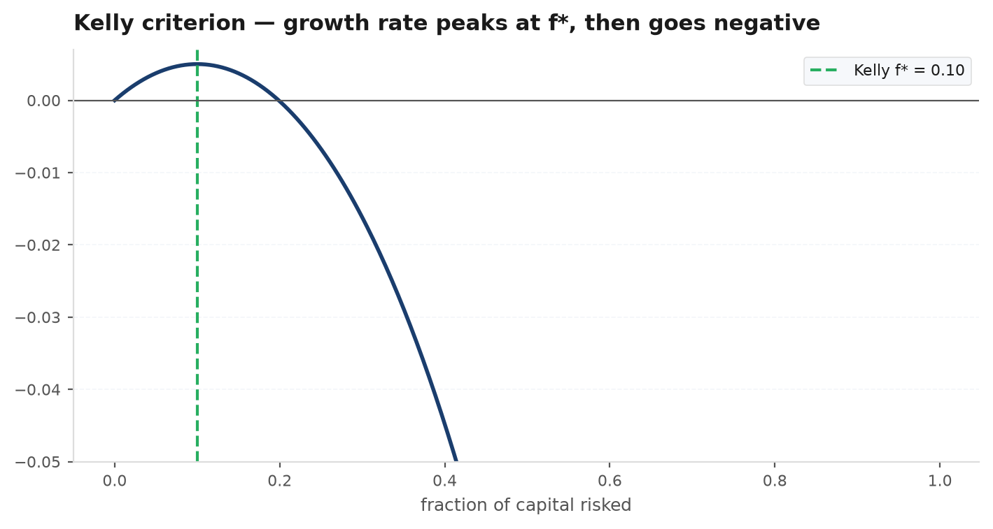
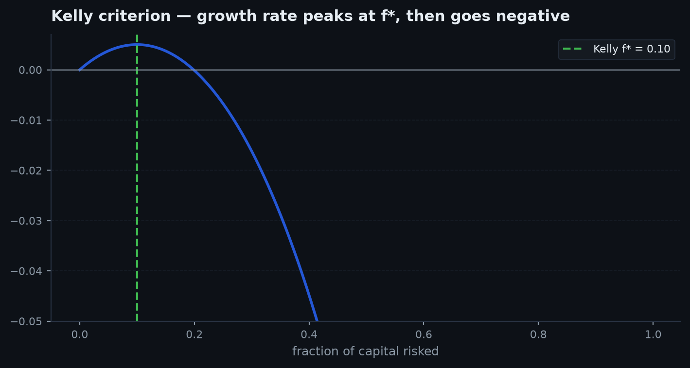
The betting escalation of Drill 12 — “you can play the game repeatedly with an edge; how much of your bankroll per play?” — is Kelly’s question: maximise $E [ln (wealth)]$ , giving $f^{*} = 2 p - 1$ for a $p$ -biased even-money coin (20% of bankroll at $p = 0.6$ ). The curve below is the entire risk-management argument in one picture: overbetting past $f^{*}$ lowers growth and eventually destroys it, which is why practitioners bet fractional Kelly — parameter uncertainty (chapter 17) makes the true $f^{*}$ lower than the estimated one.

Growth rate of wealth as a function of the fraction of bankroll bet, rising to a maximum at the Kelly fraction and then falling steeply through zero into negative growth — Long-run growth rate versus fraction of bankroll bet on a favourable game. Growth peaks at the Kelly fraction f*, is roughly flat just below it, and collapses past it — betting double-Kelly gives zero growth and beyond that ruin. The asymmetry is the answer to 'why bet less than Kelly': the penalty for overbetting is far worse than for underbetting.

Working the gauntlet: honest self-study#

A problem list only builds skill if it is used honestly. Four habits turn these twelve drills — and any problem set — into durable understanding:

Attempt cold before reading anything. Cover the solutions, give each problem a real attempt, and write down at least the classification even when stuck. Stuck is where the playbook earns its keep: name the experiment and sample space, try $n = 1$ and $n = 2$ by hand, condition on the first step, hunt for a symmetry, a martingale, a generating function. Reading a solution you have not fought for produces recognition, not ability.
Articulate the reasoning — out loud or in writing. “About 0.51 — exactly $671/1296$ — assuming a fair die and independent rolls.” Forcing the full argument into sentences exposes the gaps that silently “seeing it” hides, and separates what you derived from what you merely recalled. A recalled constant (“the answer is $e$ ”) should be flagged as recall and backed by the $1/ n!$ derivation — recall without a derivation route is exactly what fails when a parameter moves.
Simulate when — and only when — it earns its keep. Simulation is the right move to check a derived answer, to explore a variant too gnarly for closed form (three rerolls with a fee; pattern races between three players), or to settle an assumption dispute. It is the wrong move as a substitute for the two-line argument a problem is really asking for. The strongest finish: state the exact answer, then verify it — and know that the verification takes five lines:

verify_drills.py

import numpy as np

rng = np.random.default_rng(11)
trials = 200_000

# Drill 6: waiting times for HH vs HT (expect 6.0 and 4.0)
def wait(pattern):
    total = 0
    for _ in range(trials // 10):
        window, n = "", 0
        while window != pattern:
            window = (window + "HT"[rng.integers(2)])[-2:]
            n += 1
        total += n
    return total / (trials // 10)

# Drill 12: die game with k reroll options (expect 3.5, 4.25, 4.667)
def die_game(k):
    v = 3.5
    for _ in range(k):                      # V_k = E[max(X, V_{k-1})]
        rolls = rng.integers(1, 7, trials)
        v = np.maximum(rolls, v).mean()
    return v

print("HH:", wait("HH"), " HT:", wait("HT"))
print("die:", [round(die_game(k), 3) for k in (0, 1, 2)])
# HH: ~6.0  HT: ~4.0
# die: [3.5, ~4.25, ~4.67] -- matching the optionality recursion

And the fourth habit: drill for retention, not exposure. Schedule returns to the list — a week later, then a month later — and re-deriveeach answer from scratch rather than recalling it. Spaced repetition of derivations, not answers, is what moves these methods from “seen it” to “own it.” If you can still recall that HH takes 6 flips but can no longer produce the first-step equations or the ABRACADABRA argument, the drill is not done.

!The wrong answers were not random

Look back at the twelve “common wrong answers.” They are five errors wearing different costumes: adding probabilities of non-disjoint events (Drill 1), ignoring base rates and selection (Drills 2, 10), confusing the question asked with a nearby easier one (Drills 8, 11, 12), mishandling conditioning (Drill 4), and letting symmetry intuition answer an asymmetric question (Drills 6, 9). Problem setters reuse these five traps endlessly — and so do markets: every one of them has a P&L-losing twin in backtest evaluation.

Next: the series is complete. The natural continuation is the applied course, where this mathematics prices risk, sizes positions, and evaluates strategies on real data — the edgekit tutorials — or return to the series home to revisit any chapter.