Thinking in probability
Before the theorems comes a habit of mind. This chapter fixes what a probability actually is — a long-run frequency, a degree of belief, and above all a number you should be willing to bet at — and then installs the working practices that make the rest of the series land: name the experiment, write the sample space, translate percentages into natural frequencies, and simulate whenever intuition and algebra disagree. None of this is decoration. Most wrong answers in probability are not calculation errors; they are answers to a different, unstated question.
Every statement of the form “the probability of is ” can be cashed out as a price: you should be indifferent to buying or selling, at dollars, a ticket that pays $1 if happens and $0 otherwise. This single reframing does three jobs at once. It makes vague beliefs testable — would you really pay 70 cents on that ticket? It makes incoherent beliefs expensive — anyone whose prices violate the axioms can be arbitraged, as we prove below. And it connects the whole subject to markets, where prices of binary claims are crowd-sourced probability estimates. When a problem feels slippery, ask: what ticket is being priced, and what experiment settles it?
Two readings of one number#
The frequentist reading: probability is long-run relative frequency. Say the experiment can be repeated independently under identical conditions — flips of a coin, hands of a shuffled deck. Then is the value the running fraction of occurrences settles toward:
The Bayesianreading: probability is a degree of belief held by a particular agent with particular information — perfectly meaningful for one-off events (“this strategy has a real edge”, “this election goes to the incumbent”) where no repetition is available. Different agents with different information may legitimately hold different probabilities for the same event.
The crucial fact is that both readings obey the same arithmetic — the Kolmogorov axioms, stated and mined in axioms, conditioning & Bayes. Frequencies obey them because proportions do: counts of disjoint events add. Beliefs obey them because betting prices that don’t can be exploited (next section). So the machinery of this series works verbatim under either interpretation, and we will move freely between them: frequencies when we simulate, beliefs when we price an uncertain one-off. The bridge between the two — the guarantee that frequencies converge to the number beliefs should track — is the law of large numbers, proved in LLN & the CLT and visible below.
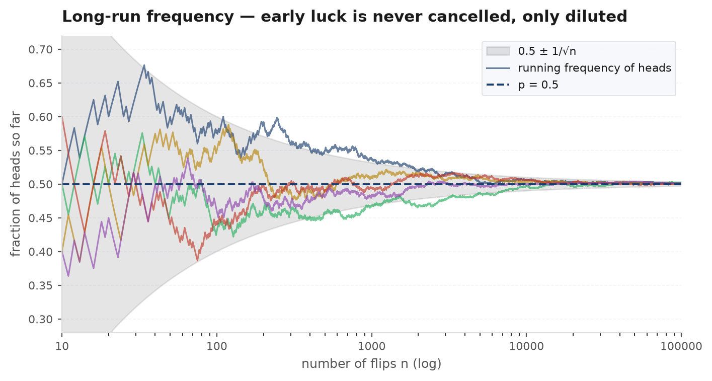
The figure is the antidote to the gambler’s fallacy before we even define independence. After five heads, tails is not “due”: the coin has no memory, and . What the law of large numbers actually promises is that the early excess — a fixed count of about heads — becomes a vanishing fraction . Absolute deviations grow like even as relative ones shrink like . Traders who “size up because the strategy is due a win” are betting on compensation, and compensation does not exist.
Odds, fair bets, and implied probability#
Betting language predates probability theory and remains the fastest way to move numbers around. Odds of against an event mean: stake to win . The conversions to memorise cold:
A bet is fair when its expected profit is zero: staking to win on an event of probability has expectation . Run the logic backwards and any quoted price becomes an implied probability: a contract paying $1 if the Fed cuts, trading at $0.62, is the market asserting . Odds of 3:1 against a horse assert .
Suppose your ticket prices violate additivity: for disjoint and you quote . An opponent sells you the two separate tickets and buys the combined one, pocketing the difference up front. At settlement the payoffs cancel exactly — in every outcome, the two small tickets together pay precisely what the big ticket pays — so the opponent’s profit is riskless. The same construction punishes and negative prices. ■ Conclusion (de Finetti): prices immune to guaranteed loss must satisfy non-negativity, normalisation and additivity — belief, if it is to be coherent, is forced into the same axioms that frequencies satisfy automatically. This is why one calculus serves both readings.
The Chevalier de Méré profitably bet even money on “at least one 6 in 4 rolls of a die”, then switched to “at least one double-6 in 24 rolls of two dice” — reasoning by proportion that made them equivalent — and started losing. Complements settle it: , while . One bet is 1.8 points above fair, the other 0.9 below — invisible over an evening, ruinous over a season, and exactly the kind of thin edge the running-frequency figure above needs thousands of trials to reveal. The correspondence between Pascal and Fermat that resolved this is the founding document of probability: the subject was born pricing bets, and this series keeps that lens.
The betting-price view is not a metaphor in finance; it is the job description. A binary option’s price is the risk-neutral probability of its event; a prediction-market contract at 62 cents is an aggregated forecast of 62%; a bookmaker’s odds grid isa probability distribution with a fee smeared across it (Problem 1 extracts the fee). Trading against a price is therefore an assertion that your probability is better than the market’s — which is why calibration, covered below, is a trader’s core competency, and why every backtest in probability & distributions for trading is ultimately a claim about whose probabilities are sharper. Edge is a probability disagreement, monetised.
Name the experiment, write the sample space#
The single most protective habit in probability: before computing anything, say precisely what is being done — the experiment — and list what can happen — the sample space . Most famous “paradoxes” are not deep; they are two parties silently using different experiments. “A family has two children and one is a boy” means one thing if a child was met at random and another if the family was selected for containing a boy — different experiments, different answers ( versus ), both computed honestly in the conditioning chapter. Until the experiment is named, the question has no answer.
Leibniz claimed 11 and 12 are equally likely totals for two dice, “since each can be made in one way”: and . The mistake is an unstated sample space of unordered pairs, which are not equally likely. The honest space is the 36 ordered outcomes, each with probability because the dice are distinct physical objects: 11 arises as or , giving , while 12 needs the single outcome : — half as likely. The lesson generalises: “equally likely” is a physical claim about the experiment, never a free assumption about whatever categories you happened to write down. Counting & combinatorics builds the systematic version: choose a space of equally likely outcomes first, then count.
Where raw intuition fails — and why#
Human probability intuition was trained on small samples and vivid stories, and it fails in patterned, predictable ways. Knowing the failure modes by name is half the cure:
- The law of small numbers.We expect small samples to look like the population. They don’t: 10 flips of a fair coin give 70%+ heads about 17% of the time. A hospital averaging 15 births a day will record far more 60%-boy days than one averaging 45 — smaller samples fluctuate more, a fact quantified by the scaling in LLN & the CLT. Every “hot streak” read off a 20-trade sample commits this error.
- Representativeness.HTHTTH looks “more random” than HHHHHH, so people call it more likely. Both are single outcomes of the same experiment, probability each. The intuition is answering a different question — how likely is a sequence of that general appearance — and Problem 4 shows that question has a respectable answer the intuition is crudely tracking. The trap is swapping questions without noticing.
- Stories over frequencies. Adding detail makes a scenario more plausible but strictly less probable: “a crash triggered by a failed bond auction” is a subset of “a crash”, yet the vivid version gets the higher number from most people (the conjunction fallacy). Monotonicity — , proved from the axioms in the next chapter — is the two-line refutation.
- Base-rate neglect.A striking piece of evidence (a positive test, a stellar backtest) swamps the boring background rate of the thing being tested for. The full accounting is Bayes’ theorem, dissected with numbers in axioms, conditioning & Bayes; the preview is that when genuine cases are rare, most alarms are false, no matter how good the alarm.
The point of cataloguing biases is not to distrust intuition wholesale — Part II of this series is devoted to building reliable intuition through symmetry, expectation tricks and limiting cases. The point is procedural: intuition proposes, arithmetic disposes. When a probability feels obvious, that feeling is data about your cognition, not about the dice. Write the sample space, or run the simulation, before the feeling hardens into an answer.
Think in natural frequencies#
Percentages are a compressed format the brain decodes badly; whole numbers of cases decode cleanly. The repair, due to Gigerenzer: restate every percentage problem as counts in a concrete population — “out of 10,000 cases…” — and watch the confusion evaporate. Take the classic screening setup (1% prevalence, 99% sensitivity, 5% false-positive rate) that defeats a majority of physicians when posed in percentages. In natural frequencies:
- Out of 10,000 people, 100 have the condition; 9,900 do not.
- Of the 100 with it, 99 test positive.
- Of the 9,900 without it, 5% — 495 — also test positive.
- So the positives number , of whom actually have the condition.
No formula was needed — the frequency format isthe computation, because it carries the base rate (100 versus 9,900) in plain sight instead of hiding it inside a conditional percentage. The habit for this series: whenever conditional probabilities tangle, drop to a population of 10,000 and count. Bayes’ theorem, when we prove it in axioms, conditioning & Bayes, will simply be this table turned into algebra.
Simulation as ground truth#
This series has a standing rule: when intuition and algebra disagree, simulate. A Monte Carlo run is an experiment — probability practised as an experimental science — and it is astonishingly cheap insurance: a five-line script settles arguments that verbal reasoning can sustain for hours. The error of a simulated probability shrinks like (the CLT again, and the same band as the coin-flip figure), so trials pins any probability to about — ample to catch every conceptual error, which tends to be off by far more. The full craft — variance reduction, convergence diagnostics, when Monte Carlo beats quadrature — is developed in Monte Carlo methods; here we establish the reflex.
A demonstration on two awkward-feeling questions. First: roll a die 10 times — what is the chance some adjacent pair of rolls is equal? Intuition flails; the algebra is a clean chain-rule product (each of the 9 gaps independently avoids a match with probability ): . Second: what is the fair price of this game — roll a die, then either keep the face value in dollars or re-roll once and keep the second roll? Optimal play re-rolls 1, 2, 3 (anything below the re-roll’s expected value ), giving . The simulation checks both:
import numpy as np

rng = np.random.default_rng(7)
trials = 200_000

# 1) P(at least one equal adjacent pair in 10 die rolls)
rolls = rng.integers(1, 7, size=(trials, 10))
has_pair = (rolls[:, 1:] == rolls[:, :-1]).any(axis=1)
exact = 1 - (5 / 6) ** 9
print(f"adjacent pair: sim {has_pair.mean():.4f}   exact 1-(5/6)^9 = {exact:.4f}")

# 2) Fair price of: roll a die, keep it, or re-roll once and keep that
first = rng.integers(1, 7, trials)
second = rng.integers(1, 7, trials)
payoff = np.where(first >= 4, first, second)   # optimal: re-roll 1, 2, 3
print(f"re-roll game:  sim {payoff.mean():.4f}   exact 17/4  = {17 / 4:.4f}")

# Monte Carlo standard error ~ sqrt(p(1-p)/n): here about 0.0009 for the
# probability — a conceptual error (wrong sample space, wrong conditioning)
# is typically 10-100x larger, so the sim catches it instantly.
Note the division of labour: the simulation does not replace the exact answer — it audits it. When the two agree to three decimals you have independent confirmation of both the algebra and the code; when they disagree, one of your two models of the experiment is wrong, and finding which is where the real learning happens. Problem 5 makes you run this loop yourself.
Calibration — making “70% confident” mean something#
If probabilities are prices, a forecaster can be audited like a market-maker. A forecaster is calibratedwhen, among all the occasions she says “70%”, the event happens about 70% of the time — and likewise at every stated level. Calibration is what elevates “70% confident” from mood to measurement: it is a frequentist property of your Bayesian utterances, the two readings of probability shaking hands.
The standard audit is the Brier score — mean squared error between forecasts and outcomes :
Worked micro-example: forecasts with outcomes score — far better than the 0.25 of a permanent fence-sitter. The Brier score is a proper scoring rule: your expected score is minimised by reporting your true belief, so it cannot be gamed by strategic exaggeration or hedging — honesty is the optimal policy, by construction. It also decomposes into calibration (are your 70%s really 70%?) plus resolution (do your forecasts actually separate the 1s from the 0s?), so the audit tells you whichskill you lack. A trading model’s predicted win probabilities deserve exactly this audit before its P&L is believed — a theme the applied series returns to with real backtests.
The road from here#
The series builds in deliberate order. First the grammar: counting & combinatoricsmakes “equally likely outcomes” a computational tool, and axioms, conditioning & Bayesturns today’s informal rules — prices must cohere, learning shrinks the sample space, base rates dominate — into theorems. Then the objects: random variables, expectation and variance, the named distributions, and joint behaviour. Then the payoff, the intuition toolkit of Part II: symmetry arguments that answer in one line what integrals answer in ten, indicator tricks, conditioning strategies, and the limit theorems — LLN & CLT — that explain when averages can be trusted. Throughout, simulation rides shotgun as the experimental check on every claimed answer. The destination is not a formula sheet; it is the ability to look at an uncertain situation, name the experiment, and price it.
Practice problems#
Five problems to test the habits before the machinery arrives — each is solvable with nothing but today’s tools: honest sample spaces, odds arithmetic, natural frequencies, and simulation.
A bookmaker quotes decimal odds of 1.80 on team A and 2.10 on team B (no draw possible). What probabilities do these prices imply, why do they sum to more than 1, and what is the bookmaker’s margin?
Solution. Implied probabilities are reciprocals: and , summing to . A coherent probability measure must sum to 1 over a partition — so these are not probabilities but prices with a fee baked in: the overround or vig, here . The Dutch book argument runs in reverse: because the quoted prices sum to more than 1, a bettor backing both sides in proportion locks in a guaranteed lossof about 3.1% — which is precisely the bookmaker’s guaranteed profit. To recover the bookmaker’s actual opinion, renormalise: and . Lesson: market prices are probability estimates plus transaction costs, and the axioms are the tool that separates the two.
You roll a fair die and are paid the face value in dollars, but you may re-roll up to two times (each re-roll discards the previous face; you must keep the last roll). What is the fair price of this game?
Solution. Work backwards from the end — the pattern behind every optimal-stopping problem. With no re-rolls left the value is . With one re-roll left, keep any face beating 3.5, i.e. 4, 5, 6: . With two re-rolls left, the continuation is worth 4.25, so keep only 5 or 6: . Fair price: , versus with one re-roll and with none. Each option adds value, but with sharply diminishing returns (, then ) — and notice the threshold rises as options remain: more optionality makes you pickier. That is the germ of option pricing, met again in the applied series.
A security screening system catches 99% of genuine threats, with a 2% false-alarm rate on innocent travellers. Genuine threats are 1 in 1,000. The system flags a traveller. Restate in natural frequencies and find the probability the traveller is a genuine threat.
Solution. Take 100,000 travellers. Genuine threats: , of whom are flagged. Innocent: , of whom 2% — — are also flagged. Total flags: , so — about 1 flag in 21, despite the “99% accurate” headline. The frequency table shows why instantly: the innocent pool is 999 times larger, so even a 2% leak from it (1,998) swamps a 99% catch from the tiny threat pool (99). Lesson: any detector of a rare condition is mostly measuring its own false-alarm rate — the theme formalised as Bayes’ theorem in the next chapter but one.
A fair coin is flipped six times. (a) Which is more likely: HTHTTH or HHHHHH? (b) Which is more likely: a sequence with three heads and three tails in some order, or a sequence with six heads? Explain why honest answers to (a) and (b) differ.
Solution. (a) Equally likely. Each specific length-6 sequence is a single outcome of the sample space of equally likely strings: apiece. (b) Now the events are setsof outcomes: “three of each” contains strings, probability , versus for the single all-heads string — twenty times more likely. The representativeness illusion is the brain silently answering (b) when asked (a): HTHTTH gets credit for the 19 siblings that share its look. Both intuitions are correct answers — to different questions about different events in the same sample space. Lesson: an unstated sample space, or an unstated event, is where wrong answers are manufactured; name both and the paradox dissolves.
Two dice are rolled repeatedly. What is the probability a sum of 7 appears before a sum of 8? Design the Monte Carlo estimate, predict its standard error at trials, and verify against the exact answer.
Solution. Simulation design: one trial = roll pairs until the sum is 7 or 8; record a win on 7. Loop trials, report the win fraction. (Vectorised shortcut: rolls with sums other than 7 or 8 are irrelevant, so equivalently draw from the conditional distribution over decisive rolls only.) Exact answer: that same observation done analytically — only the first decisive roll matters, and among decisive sums, vs , so . Error budget: , so the simulation should land within about of — if it reads 0.58, the code is wrong, not the luck. Lesson: a simulation is only evidence once you have predicted its error bar; and the analytic trick — condition on the first decisive trial and ignore the rest — is the renormalisation idea that powers conditioning and, much later, craps and first-passage problems in Monte Carlo methods.
Next:the “equally likely outcomes” promise gets its engine — permutations, combinations, and the art of counting without listing: Counting & combinatorics.