Counting & combinatorics

Almost every discrete probability question reduces to counting: favourable outcomes over total outcomes, when outcomes are equally likely. This chapter builds the counting toolkit — the multiplication rule, permutations and combinations, the binomial theorem, stars and bars, inclusion–exclusion, derangements, and the symmetry arguments that turn pages of algebra into one-line answers. It closes with the birthday problem, the first of many places where a quiet exponential sneaks up on your intuition.

✦Intuition — why counting comes first

The classical definition of probability — $P (A) = ∣ A ∣/∣Ω∣$ for equally likely outcomes — makes probability literally a counting problem. Classic problems cluster in this territory because it has no formulas to hide behind: either you can decompose the outcome space cleanly or you cannot. The entire skill is choosing the right decomposition — ordered or unordered, with or without replacement, direct count or complement count — and the tools below are exactly that menu.

The multiplication rule and ordered selection#

The multiplication rule is the atom of counting: if a procedure has $k$ stages and stage $i$ can be completed in $n_{i}$ ways regardless of the earlier choices, the whole procedure has $n_{1} n_{2} \dots n_{k}$ outcomes. Everything else in this chapter is this rule plus bookkeeping.

An ordered selection of $k$ distinct items from $n$ is a permutation. The first slot has $n$ choices, the second $n - 1$ , and so on:

P (n, k) = n (n - 1) \dots (n - k + 1) = \frac{n !}{( n - k )!}, P (n, n) = n!

✦Worked example — arranging a watchlist

Display 3 of 8 instruments in ranked dashboard slots: $P (8, 3) = 8 \cdot 7 \cdot 6 = 336$ arrangements. Rank all 8 and it is $8! = 40, 320$ — factorials explode, which is why brute-force enumeration dies fast and clever counting matters.

Combinations and the binomial theorem#

When order does not matter, we are counting combinations — subsets of size $k$ . The derivation is a deliberate overcount-then-divide: each unordered subset of size $k$ appears exactly $k!$ times among the ordered selections (once per internal ordering), so

(k n) = \frac{P ( n , k )}{k !} = \frac{n !}{k ! ( n - k )!} .

Two identities do most of the work in practice. Symmetry, $(k n) = (n - k n)$ , because choosing which $k$ to include is the same as choosing which $n - k$ to exclude. And Pascal’s identity:

(k n) = (k - 1 n - 1) + (k n - 1) .

✦Proof — Pascal's identity by conditioning on one element

Fix a particular element, say item $n$ . Every size- $k$ subset either contains it or not. Subsets that contain it are completed by choosing $k - 1$ of the remaining $n - 1$ : $(k - 1 n - 1)$ ways. Subsets that avoid it choose all $k$ from the other $n - 1$ : $(k n - 1)$ ways. The two cases are disjoint and exhaustive, so they add. ■This “condition on one element” move is a template — the same trick proves many binomial identities without algebra.

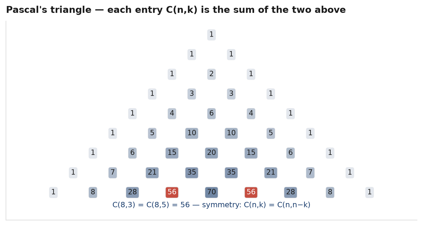
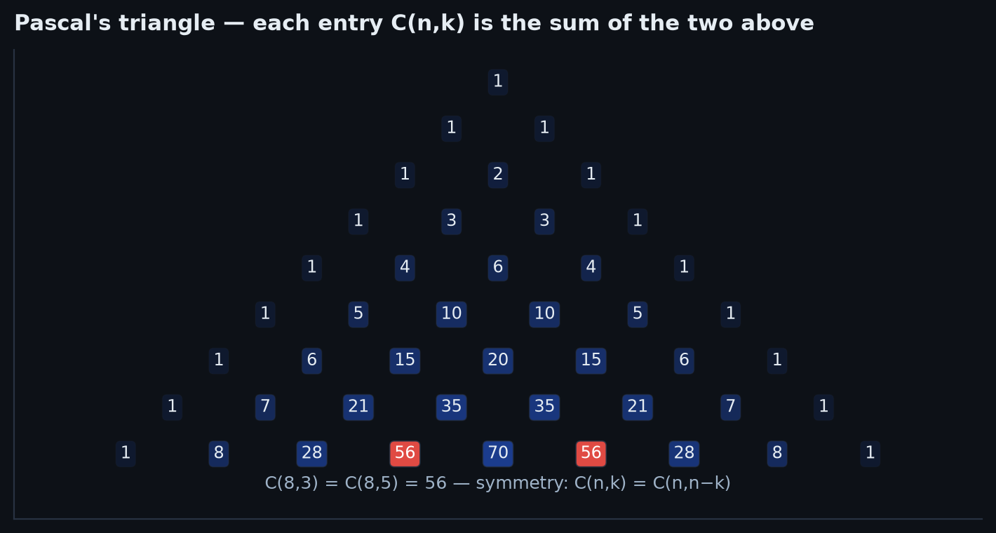
Pascal's triangle with binomial coefficients, highlighting how each entry is the sum of the two above it — Pascal's triangle: row n lists C(n,0) … C(n,n), and each entry is the sum of the two above it — Pascal's identity made visual. The rows also sum to 2^n (every subset is in or out) and, normalised, converge to the binomial distribution's bell shape.

The binomial theorem is the algebraic face of the same count:

(x + y)^{n} = k = 0 \sum n (k n) x^{k} y^{n - k} .

✦Proof sketch — binomial theorem by choosing factors

Expand $(x + y)^{n}$ as a product of $n$ brackets. Each term in the expansion picks either $x$ or $y$ from every bracket, so a term equal to $x^{k} y^{n - k}$ arises once for every choice of which $k$ brackets contribute the $x$ — and there are exactly $(k n)$ such choices. ■ Setting $x = y = 1$ gives $\sum_{k} (k n) = 2^{n}$ (every element in or out), and $x = p, y = 1 - p$ shows binomial probabilities sum to 1 — the distribution you will meet properly in the distribution zoo.

✦Worked example — committee counts by hand

From 12 analysts, how many ways to form a research pod of 4? $(4 12) = \frac{12 \cdot 11 \cdot 10 \cdot 9}{4 !} = \frac{11 , 880}{24} = 495$ . If the pod must contain exactly 2 of the 5 seniors (and so 2 of the 7 juniors), count each group independently and multiply: $(2 5) (2 7) = 10 \cdot 21 = 210$ . The multiplication rule glues independent sub-counts together.

Stars and bars#

How many ways can you place $n$ identical items into $k$ labelled boxes — equivalently, how many non-negative integer solutions has $x_{1} + x_{2} + \dots + x_{k} = n$ ? The answer:

(k - 1 n + k - 1) .

✦Proof — the stars-and-bars bijection

Write the $n$ items as stars and insert $k - 1$ bars to cut the row into $k$ segments; segment $i$ ’s star-count is $x_{i}$ . For example $⋆ ⋆ ∣ ⋆ ∣ ∣ ⋆$ encodes $(2, 1, 0, 1)$ . Every arrangement of $n$ stars and $k - 1$ bars corresponds to exactly one solution and vice versa, and arranging them means choosing which $k - 1$ of the $n + k - 1$ positions hold bars: $(k - 1 n + k - 1)$ . ■ For strictly positive solutions ( $x_{i} \geq 1$ ), first give each box one star, leaving $n - k$ free: $(k - 1 n - 1)$ .

✦Worked example — allocating risk units

You have 10 identical 1R risk units to spread across 4 strategies (a strategy may get zero). Solutions of $x_{1} + x_{2} + x_{3} + x_{4} = 10$ : $(3 13) = 286$ allocations. Require every strategy to get at least one unit and it drops to $(3 9) = 84$ . Which allocation is best is a sizing question (the math of edge); sizing the search space is where any grid search starts.

Inclusion–exclusion#

Unions are awkward because events overlap; inclusion–exclusion corrects the double counting. For two and three events:

P (A \cup B) = P (A) + P (B) - P (A \cap B),

P (A \cup B \cup C) = P (A) + P (B) + P (C) - P (A B) - P (A C) - P (B C) + P (A B C),

and in general, for events $A_{1}, \dots, A_{n}$ :

P (i = 1 ⋃ n A_{i}) = i \sum P (A_{i}) - i < j \sum P (A_{i} A_{j}) + i < j < k \sum P (A_{i} A_{j} A_{k}) - \dots + (- 1)^{n + 1} P (A_{1} \dots A_{n}) .

✦Proof — two sets exactly, general case by counting an element

Two sets. Decompose the union into disjoint pieces: $A \cup B = (A ∖ B) \cup (B ∖ A) \cup (A \cap B)$ . Additivity over disjoint events gives $P (A \cup B) = P (A ∖ B) + P (B ∖ A) + P (A B)$ . Since $P (A) = P (A ∖ B) + P (A B)$ and similarly for $B$ , substituting yields $P (A) + P (B) - P (A B)$ . ■

General case (sketch). Take an outcome belonging to exactly $m \geq 1$ of the events. On the left it is counted once. On the right it is counted $(1 m) - (2 m) + (3 m) - \dots$ times, and by the binomial theorem applied to $0 = (1 - 1)^{m}$ this alternating sum equals exactly 1. Every outcome is counted once on both sides, so the identity holds. ■

✦Worked example — divisible by 2 or 3

How many integers in ${1, \dots, 100}$ are divisible by 2 or 3? Multiples of 2: 50. Multiples of 3: 33. Multiples of 6 (counted twice): 16. Total: $50 + 33 - 16 = 67$ . Note the rhythm — add the singles, subtract the pairs — which scales mechanically to any number of conditions.

Truncating the alternating sum after the first term gives the union bound $P (\cup_{i} A_{i}) \leq \sum_{i} P (A_{i})$ — proved properly in the axioms chapter and the engine behind Bonferroni corrections in multiple testing.

Derangements and the 1/e law#

A derangement is a permutation with no fixed point — $n$ people toss their hats in a pile, each takes one back at random, and nobody gets their own. Let $D_{n}$ count them. Inclusion–exclusion cracks this in three lines.

✦Proof — counting derangements, and the limit 1/e

Let $A_{i}$ be the event that person $i$ gets their own hat. We want the complement of $\cup_{i} A_{i}$ . Any intersection of $k$ specific $A_{i}$ ’s fixes those $k$ hats and permutes the rest freely: $(n - k)!$ permutations, and there are $(k n)$ ways to pick which $k$ . So by inclusion–exclusion,

D_{n} = k = 0 \sum n (- 1)^{k} (k n) (n - k)! = n! k = 0 \sum n \frac{( - 1 ) ^{k}}{k !} .

The sum is the partial Taylor series of $e^{- 1}$ , so

\frac{D _{n}}{n !} = k = 0 \sum n \frac{( - 1 ) ^{k}}{k !} ⟶ \frac{1}{e} \approx 0.3679. ■

Convergence is astonishingly fast — the error is below $1/ (n + 1)!$ . The chance that at least one person gets their own hat is $1 - 1/ e \approx 0.632$ — a constant worth memorising; it reappears as the chance an observation enters a bootstrap resample in resampling.

n	D_n	D_n / n!
3	2	0.3333
4	9	0.3750
6	265	0.3681
10	1,334,961	0.36788 (1/e to 5 dp)

Symmetry arguments#

The fastest counting is the counting you avoid. A symmetry argument notes that the random mechanism treats certain outcomes identically, so their probabilities must be equal — no enumeration needed.

Any position is as good as the first. Shuffle a deck: the probability the 17th card is an ace is $4/52$ , same as the first — the shuffle is exchangeable, so every position sees the same marginal distribution.
Relative order is uniform. Among $k$ distinct exchangeable draws, all $k!$ orderings are equally likely — the germ of order statistics and of the fact that a record at time $n$ has probability $1/ n$ .
Pair up outcomes.A random walk’s paths reflect into equally likely mirror paths — the reflection principle of random walks & Brownian motion is a symmetry argument in disguise.

✦Worked example — second ace, by symmetry

Deal two cards. What is $P (second card is an ace)$ ? The brute-force way conditions on the first card: $\frac{4}{52} \cdot \frac{3}{51} + \frac{48}{52} \cdot \frac{4}{51} = \frac{12 + 192}{2652} = \frac{204}{2652} = \frac{1}{13}$ . The symmetry way: the second card is a uniformly random card, so $4/52 = 1/13$ . Same answer, zero algebra. The best practice questions are deliberately set up so the conditional route is a slog and the symmetry route is one sentence.

The birthday problem#

Among $n$ people with uniformly random birthdays over 365 days, what is the chance two share a birthday? Count the complement — all birthdays distinct — with the multiplication rule:

P (no match) = i = 0 \prod n - 1 \frac{365 - i}{365} = i = 1 \prod n - 1 (1 - \frac{i}{365}) .

✦Derivation — the exponential approximation

Take logs and use $ln (1 - x) \approx - x$ for small $x$ :

ln P (no match) = i = 1 \sum n - 1 ln (1 - \frac{i}{365}) \approx - i = 1 \sum n - 1 \frac{i}{365} = - \frac{n ( n - 1 )}{2 \cdot 365} .

So the collision probability is approximately

P (match) \approx 1 - exp (- \frac{n ( n - 1 )}{730}) \approx 1 - e^{- n^{2} /730} .

Setting this to $1/2$ gives $n \approx 730 ln 2 \approx 22.5$ — hence the famous answer 23. The mechanism: the number of pairs grows like $n^{2} /2$ — with 23 people there are already $(2 23) = 253$ chances to collide. Intuition tracks $n$ ; probability tracks $n^{2}$ . Exact values: $0.5073$ at $n = 23$ , $0.9704$ by $n = 50$ .

Probability of at least one shared birthday versus group size, crossing 50 percent near 23 people, with the exponential approximation overlaid — The birthday problem: exact collision probability (solid) against group size, with the 1 − exp(−n(n−1)/730) approximation (dashed) nearly on top of it. The curve crosses 1/2 at n = 23 and is nearly certain by 60 — pair counts grow quadratically, so collisions arrive far earlier than linear intuition expects.

→Quant lens — backtest collisions and the combinatorics of overfitting

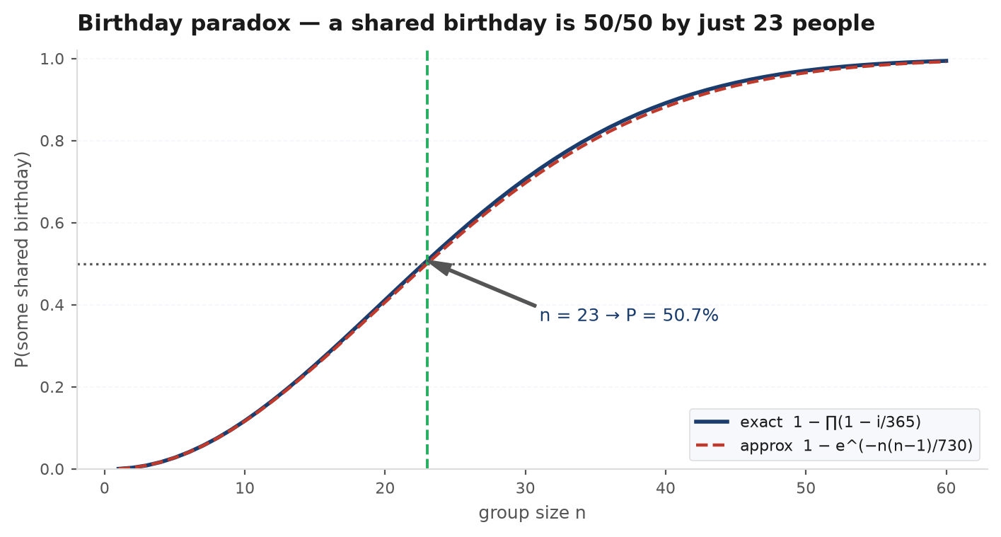
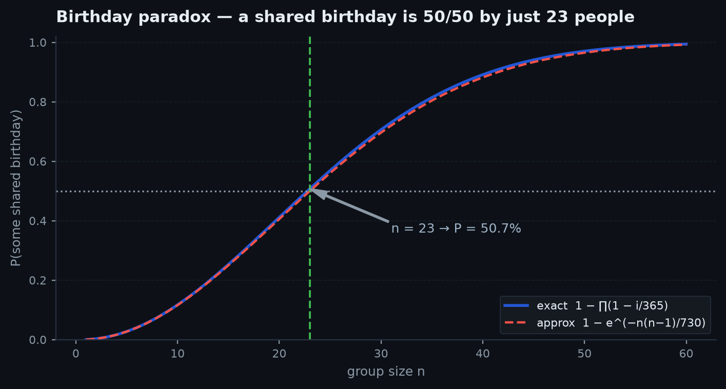
The birthday effect is the statistical heart of data snooping: test many strategy variants and the implicit comparisons grow combinatorially, so “surprising” coincidences become near-certain by chance. A grid of 5 entry rules × 6 exit rules × 10 lookbacks is already $300$ strategies by the multiplication rule; the expected maximum Sharpe among them grows like $2 ln N$ even when every strategy is pure noise. The counting above is how you size the search space you actually explored — the first number an honest backtest audit asks for, and the input to the corrections in multiple testing & paradoxes.

Simulation confirms both headline constants — the $50.7%$ birthday collision at $n = 23$ and the $1/ e$ derangement law:

counting_checks.py

import numpy as np

rng = np.random.default_rng(11)
trials = 200_000

# --- Birthday problem: P(shared birthday) among n = 23 people ---
n = 23
bdays = rng.integers(0, 365, size=(trials, n))
s = np.sort(bdays, axis=1)
collide = (np.diff(s, axis=1) == 0).any(axis=1)
print(f"P(match), n=23:  {collide.mean():.4f}   (exact 0.5073)")

# --- Derangements: P(no fixed point) for a random permutation, n = 10 ---
m = 10
perms = np.argsort(rng.random((trials, m)), axis=1)   # uniform random permutations
no_fixed = ~(perms == np.arange(m)).any(axis=1)
print(f"P(derangement):  {no_fixed.mean():.4f}   (1/e = {1/np.e:.4f})")

Sampling with and without replacement#

The last distinction the toolkit needs: does a draw change the pool? Draw $n$ items from a population of $N$ containing $K$ “successes.”

With replacement — draws are independent, each a success with probability $p = K / N$ . The success count is binomial: $P (X = k) = (k n) p^{k} (1 - p)^{n - k}$ .
Without replacement — draws deplete the pool and are dependent. The count is hypergeometric, a pure ratio of combination counts: $P (X = k) = (k K) (n - k N - K) / (n N)$ — choose which successes, choose which failures, over all ways to choose the sample.

Both have mean $n p$ , but the hypergeometric variance carries the finite-population correction $\frac{N - n}{N - 1}$ — sampling without replacement is less variable, because each draw removes what you drew. When $N ≫ n$ the correction vanishes and the two coincide. Both distributions get full treatment in the distribution zoo.

✦Worked example — at least one ace in a 5-card hand

Complement count: $P (no ace) = (5 48) / (5 52) = \frac{1 , 712 , 304}{2 , 598 , 960} \approx 0.6588$ , so $P (at least one ace) \approx 0.3412$ . The pattern — “at least one” means complement of “none” — is the single most-used move in counting problems.

Practice problems#

Six classics — note how often the slick answer is a complement, a symmetry, or a division by an overcount.

→Problem 1 — Handshakes

At a meeting of $n$ people, everyone shakes hands with everyone else exactly once. How many handshakes? If there were 66 handshakes, how many people attended?

Solution. A handshake is an unordered pair of people: $(2 n) = \frac{n ( n - 1 )}{2}$ . (Slick double-count: each of $n$ people shakes $n - 1$ hands, and each shake is counted twice — divide by 2.) For 66: $n (n - 1) = 132 = 12 \cdot 11$ , so $n = 12$ . Notice this is the same $(2 n)$ that counts pairwise correlations in an $n$ -asset portfolio and pairwise collisions in the birthday problem.

→Problem 2 — Splitting into two teams

How many ways can 10 people be split into two teams of 5?

Solution. The trap is $(5 10) = 252$ . That counts labelledteams (“team A gets these five”) — but choosing five people for team A and choosing their five complements produce the same split. Each unlabelled split is counted twice, so the answer is $252/2 = 126$ . Generalisation worth stating aloud: $m$ unlabelled groups of $k$ give $(mk)! / ((k!)^{m} m!)$ . Overcount-then-divide, again.

→Problem 3 — De Méré's bet: at least one six

Which is more likely: at least one 6 in 4 rolls of a die, or at least one double-6 in 24 rolls of two dice?

Solution. Complements. $P_{1} = 1 - (5/6)^{4} = 1 - 0.4823 = 0.5177$ , while $P_{2} = 1 - (35/36)^{24} = 1 - 0.5086 = 0.4914$ . The first bet wins in the long run; the second loses — the discrepancy that sent de Méré to Pascal and Fermat. The naive intuition $4 \cdot \frac{1}{6} = 24 \cdot \frac{1}{36}$ fails because probabilities of unions are not sums — inclusion–exclusion is exactly the ignored correction.

→Problem 4 — The hat-check (derangement) problem

100 traders leave badges at reception; the receptionist hands them back uniformly at random. What is the probability nobody receives their own badge? What is the expected number who do?

Solution. From the derangement derivation above, $P (nobody matches) = D_{100} /100! = \sum_{k = 0}^{100} (- 1)^{k} / k! \approx 1/ e \approx 0.3679$ — effectively exact at $n = 100$ . For the expected number of matches, use indicators: $X = \sum_{i} 1_{i}$ with $P (1_{i} = 1) = 1/100$ , so $E [X] = 100 \cdot \frac{1}{100} = 1$ — exactly one match on average, for any $n$ , despite the dependence between indicators. That trick gets a full section in random variables & moments.

→Problem 5 — Count the full houses

How many 5-card poker hands are a full house (three of one rank, two of another), and what is the probability?

Solution. Build the hand by stages with the multiplication rule: choose the trip rank (13), its three suits ( $(3 4) = 4$ ), the pair rank (12 — order matters here because trip-rank and pair-rank play different roles), its two suits ( $(2 4) = 6$ ): $13 \cdot 4 \cdot 12 \cdot 6 = 3744$ hands. Probability: $3744/ (5 52) = 3744/2, 598, 960 \approx 0.00144$ , about 1 in 694. The classic error is using $(2 13)$ for the ranks — that treats trip-rank and pair-rank as interchangeable, and they are not: KKK-QQ and QQQ-KK are different hands.

→Problem 6 — Birthday variants

(a) How many people are needed for a 50% chance someone shares your birthday? (b) Roughly how many for a 50% chance of a three-way birthday collision?

Solution. (a) This is not 23 — matching a fixed day kills the quadratic pair effect. $P (no match to you) = (364/365)^{n}$ ; setting it to $1/2$ gives $n = ln 2/ ln (365/364) \approx 253$ . Ten times more people, because only $n$ comparisons are available rather than $(2 n)$ . (b) Triples scale as $(3 n) \sim n^{3} /6$ , each hitting with probability $1/36 5^{2}$ ; the count reaches coin-flip territory around $n \approx 88$ (the exact answer). Say the takeaway out loud: what counts as a coincidence sets the exponent, and the exponent determines everything.

Next: counting handles equally likely outcomes; axioms, conditioning, and Bayes handle everything else. Axioms, conditioning & Bayes.