Expectation & the linearity trick

Random variables & moments defined expectation and stated its one superpower: linearity, with no independence required. This chapter is the deep dive on that superpower — the single most productive computational idea in probability. The method is three steps long: decompose a count into indicators, take expectations, add. It computes in one line what distributions take pages to describe — hat-check matches, birthday collisions, records, runs, coupon collections — and it extends to second moments and to a tail-sum formula that reads means off survival curves. By the end you should reach for indicators reflexivelywhenever a question begins “what is the expected number of…”.

✦Intuition — averages commute with everything; distributions commute with nothing

Most operations in probability fight you: the distribution of a sum is a convolution, the maximum of two variables has a new CDF, dependence tangles every joint computation. Expectation is the exception — it slides through sums untouched, whatever the dependence between the pieces. So the winning move is to rewrite your quantity as a sum of the simplest possible pieces — indicators, which are events wearing a 0/1 costume. A complicated random count is a pile of tiny yes/no questions, and the expected count is the sum of their yes-probabilities. You never need to know how the answers correlate — until you ask about spread or tails, when the correlations come storming back (the closing warning below).

Centre of mass, fair price#

Two pictures of $E [X]$ are worth keeping, beyond the defining formula in random variables & moments. First, centre of mass: place weight $p (x)$ at each point $x$ , and $E [X]$ is where the line balances. Balance points respond linearly to shifting and scaling the masses — why linearity should feel inevitable — and they chase outliers: a tiny mass placed far out moves the balance point a long way, the geometric seed of every fat-tail pathology in LLN & CLT.

Second, fair price: $E [X]$ is the unique price at which a ticket paying the random amount $X$ is a break-even trade in the long run — charge more and the seller wins on average, less and the buyer does. This is the sense in which expectation prices a gamble with a single number, and it is the licence behind every expectancy computation on a trading desk: a strategy’s worth per trade is $E [PnL]$ , full stop (the math of edge). The caveats — infinite means, and the fact that a fair price says nothing about the ride — are refinements; the fair-price reading is the anchor.

Linearity: the theorem that asks for nothing#

For any random variables $X_{1}, \dots, X_{n}$ with finite means and any constants $a_{1}, \dots, a_{n}$ :

E [a_{1} X_{1} + \dots + a_{n} X_{n}] = a_{1} E [X_{1}] + \dots + a_{n} E [X_{n}] .

No independence. No identical distributions. No assumptions about the joint behaviour at all. The proof (given in full in random variables & moments) is one rearrangement: write the expectation of the sum against the joint distribution, split the sum, and observe that each term only ever consults its own marginal — the joint distribution, where all the dependence lives, gets summed out before it can matter.

✦Why this is genuinely shocking

Every other summary of a sum depends on the dependence: $Var (X + Y)$ needs the covariance, the distribution of $X + Y$ needs the entire joint law, $E [max (X, Y)]$ and $E [X Y]$ both move when correlation moves. The mean of a sum alone is immune, and that immunity makes the indicator method a method: carve a count into overlapping, entangled, perfectly correlated pieces — however the problem makes convenient — and the expected total still adds up. When a computation feels blocked because “the events aren’t independent,” that instinct is the bug: for expectations, dependence is never an obstruction.

The indicator method, as a recipe#

An indicator $1_{A}$ equals 1 when $A$ occurs and 0 otherwise, so $E [1_{A}] = 1 \cdot P (A) + 0 \cdot P (A^{c}) = P (A)$ — expectations of indicators are probabilities. The recipe:

Step 1 — decompose. Recognise your quantity as a count and write $X = \sum_{i = 1}^{n} 1_{A_{i}}$ , where $A_{i}$ = “the $i$ -th potential contributor actually contributes.”
Step 2 — take expectations. Linearity: $E [X] = \sum_{i} P (A_{i})$ — each a one-event probability, usually easy, often by symmetry.
Step 3 — sum. Frequently all $P (A_{i})$ are equal and the answer is $n \cdot P (A_{1})$ .

The craft is entirely in Step 1: choosing what to index — items (fixed points), pairs (collisions, inversions), positions (records, runs, patterns), boxes (empty cells), or stages of a process (coupon collector). Everything after that choice is arithmetic.

Five classics, fully worked#

✦Worked example — the hat-check problem

$n$ people leave hats at a party; the hats come back in uniformly random order. Expected number of correct returns? Index the people: $A_{i}$ = “person $i$ gets hat $i$ .” Hat $i$ is equally likely to land on any of the $n$ heads, so $P (A_{i}) = 1/ n$ and

E [X] = i = 1 \sum n \frac{1}{n} = 1 for every n .

One expected match whether $n = 3$ or a million — a surprising invariance, delivered without touching the ferociously dependent joint structure (person 1 matching changes everyone else’s chances). Contrast the distributional question “what is $P (X = 0)$ ?” — the derangement problem, which needs full inclusion–exclusion (counting & combinatorics) to reach $\approx 1/ e$ .

✦Worked example — birthday collisions

$n$ people, 365 equally likely birthdays. Expected number of pairs sharing a birthday? Index the pairs: $(2 n)$ of them, each sharing with probability $1/365$ (whatever the first person’s birthday, the second matches it with probability $1/365$ ):

E [collisions] = (2 n) \frac{1}{365} = \frac{n ( n - 1 )}{730} .

At $n = 23$ : $\frac{23 \cdot 22}{730} = \frac{506}{730} \approx 0.693$ — crossing $ln 2$ exactly where the birthday probability crosses $1/2$ . No coincidence: for rare, roughly independent events, $P (none) \approx e^{- E [count]}$ — the heuristic developed in balls, bins & birthdays.

✦Worked example — records in a random sequence

Observe $n$ i.i.d. continuous values (no ties); position $i$ sets a record if it exceeds everything before it. By symmetry each of the first $i$ values is equally likely to be their largest, so $P (record at i) = 1/ i$ and

E [records] = 1 + \frac{1}{2} + \frac{1}{3} + \dots + \frac{1}{n} = H_{n} \approx ln n + 0.5772.

A century of daily data ( $n \approx 25, 000$ ) should produce only $H_{25000} \approx 10.7$ record highs under the i.i.d. null — records are logarithmically rare. The indicators are dependent and non-identically distributed; linearity does not blink.

✦Worked example — runs in coin flips

Flip a fair coin $n$ times; a run is a maximal block of equal outcomes (HHTHH has runs HH, T, HH). Index the boundaries: a new run starts at flip 1, and at flip $i \geq 2$ exactly when it differs from flip $i - 1$ — probability $1/2$ :

E [runs] = 1 + (n - 1) \cdot \frac{1}{2} = \frac{n + 1}{2} .

100 flips: 50.5 runs expected. Eyeballed randomness looks streaky — a “hot regime” narrative fits almost any fair sequence — and comparing observed runs to $(n + 1) /2$ is precisely the runs test for serial dependence.

And a preview: throw $n$ balls into $n$ boxes uniformly. Indexing the boxes, each is empty with probability $(1 - \frac{1}{n})^{n}$ , so the expected number of empty boxes is $n (1 - \frac{1}{n})^{n} \to n / e \approx 0.368 n$ — the opening move of the occupancy theory in balls, bins & birthdays.

→Quant lens — expected counts run the shop

Operational questions on a desk are expected-count questions, and linearity answers them without a correlation model: expected positions hitting stops today = sum of per-position stop probabilities; expected strategies in a 200-strategy scan clearing a Sharpe threshold by luck = 200 × (false positive rate) — the arithmetic of multiple testing & paradoxes. All exact under arbitrary dependence. What dependence changes is the distribution aroundthe count: correlated stops fire together, so a mean of 5 stop-outs can mean “5 most days” or “0 most days, 50 in a crash.” Means for free, tails at a price.

Coupon collector, by stage decomposition#

Indicators decompose counts; the same linearity decomposes durations. How many uniform draws from $n$ coupon types until you own all $n$ ? Stage $k$ begins when you hold $k - 1$ distinct types and ends when a new one arrives; during it each draw is new with probability $p_{k} = \frac{n - k + 1}{n}$ , so the stage length is geometric with mean $n / (n - k + 1)$ , and linearity glues the stages:

E [T] = k = 1 \sum n \frac{n}{n - k + 1} = n (\frac{1}{n} + \dots + \frac{1}{2} + 1) = n H_{n} \approx n ln n .

For $n = 52$ : $52 H_{52} \approx 52 \times 4.538 \approx 236$ draws to see every card. The stage lengths happen to be independent, but the proof never used that — only that the total is a sum of stages with known means. The harder cousins (unequal coupon probabilities, collect two of each) live in probability brainteasers; stage decomposition is the move that opens all of them.

The tail-sum formula#

For a non-negative integer-valued $X$ , the mean can be read off the survival function — no PMF required:

E [X] = k = 1 \sum \infty P (X \geq k), and continuously, E [X] = \int_{0}^{\infty} P (X > t) d t (X \geq 0) .

✦Proof — double counting, i.e. indicators again

The formula is the indicator method applied to thresholds: $X$ clears exactly $X$ of the thresholds $1, 2, 3, \dots$ , so $X = \sum_{k \geq 1} 1 {X \geq k}$ . Take expectations — linearity is safe for non-negative terms — and each indicator surrenders its probability:

E [X] = k \geq 1 \sum E [1 {X \geq k}] = k \geq 1 \sum P (X \geq k) . ■

The picture is a double count: stack a bar of height $n$ with mass $P (X = n)$ ; summing bar by bar gives $\sum n P (X = n)$ , summing layer by layer gives $\sum_{k} P (X \geq k)$ — same area, two slicings. The continuous version is the same swap with Fubini: the mean is the area under the survival curve.

Two showcase uses. The geometric: $P (X \geq k) = (1 - p)^{k - 1}$ , so $E [X] = \sum_{k \geq 1} (1 - p)^{k - 1} = 1/ p$ — two lines, no power-series differentiation. Better still, the expected maximum $M$ of $n$ fair dice, where the survival form is natural because maxima have easy CDFs: $P (M \geq k) = 1 - P (all < k) = 1 - (\frac{k - 1}{6})^{n}$ , so

E [M] = k = 1 \sum 6 [1 - (\frac{k - 1}{6})^{n}] = 6 - \frac{1 ^{n} + 2 ^{n} + \dots + 5 ^{n}}{6 ^{n}} .

For $n = 2$ : $6 - \frac{1 + 4 + 9 + 16 + 25}{36} = 6 - \frac{55}{36} = \frac{161}{36} \approx 4.47$ ; for $n = 10$ , $\approx 5.86$ . Whenever $P (X \geq k)$ is easier than $P (X = k)$ — maxima, waiting times, survival processes — the tail-sum route wins; it is also the identity that finishes Wald’s theorem in martingales & optional stopping.

Second moments: the method extends to pairs#

Squaring a sum of indicators produces indicator pairs, and $1_{A_{i}} 1_{A_{j}} = 1_{A_{i} \cap A_{j}}$ — linearity reaches second moments too:

E [X^{2}] = E [i \sum j \sum 1_{A_{i}} 1_{A_{j}}] = i \sum P (A_{i}) + i \neq = j \sum P (A_{i} \cap A_{j}) .

The diagonal terms reproduce $E [X]$ (indicators square to themselves); the off-diagonal terms need pairwisejoint probabilities — dependence’s first, limited, appearance, and still far less than the full joint law.

✦Worked example — the hat-check count has variance 1

For the hat-check $X$ : $P (A_{i}) = 1/ n$ , and for $i \neq = j$ , $P (A_{i} \cap A_{j}) = \frac{1}{n} \cdot \frac{1}{n - 1}$ (hat $i$ home, then hat $j$ home among the remaining $n - 1$ ). With $n$ diagonal and $n (n - 1)$ off-diagonal terms:

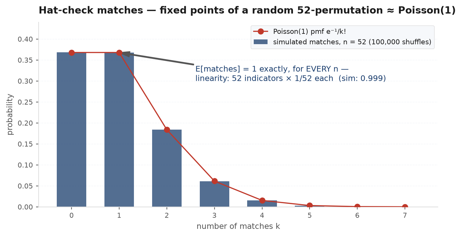
E [X^{2}] = n \cdot \frac{1}{n} + n (n - 1) \cdot \frac{1}{n ( n - 1 )} = 1 + 1 = 2, Var (X) = 2 - 1^{2} = 1.

Mean 1, variance 1, for every $n \geq 2$ — and in the limit the count converges to Poisson(1): $P (X = k) \to e^{- 1} / k!$ , about 36.8% chance of no match, 36.8% of exactly one, 18.4% of two (Poisson processes).

Histogram of the number of fixed points of a random permutation of 52 items matching the Poisson(1) probabilities, with the mean marked at exactly 1 — The hat-check count for n = 52: simulated matches (bars) against Poisson(1) (markers), mean pinned at exactly 1 — as it is for every n. Linearity delivered that mean in one line; pinning down the full distribution took inclusion–exclusion, factorial moments, and a Poisson limit theorem. Means are cheap, distributions are expensive.

Symmetry × linearity: expected positions#

The most elegant applications pair linearity with a symmetry argument that makes every $P (A_{i})$ obvious. The canonical example: in a shuffled 52-card deck, how many cards come before the first ace, on average?

✦Worked example — 48/5 cards before the first ace

Index the 48 non-aces: $A_{i}$ = “non-ace $i$ lies before all four aces.” The relative order of five specific cards — non-ace $i$ and the four aces — is uniform over the $5!$ arrangements, so non-ace $i$ comes first with probability $1/5$ . Hence

E [cards before first ace] = 48 \cdot \frac{1}{5} = \frac{48}{5} = 9.6,

and the first ace sits at expected position $9.6 + 1 = 10.6 = 53/5$ . The equivalent picture: the four aces split the other 48 cards into 5 exchangeable gaps, each holding $48/5$ cards on average. Spacing arguments of this kind are developed properly in symmetry & exchangeability and order statistics.

Simulation check#

Two headline results — hat-check mean and variance both exactly 1, and records growing like $H_{n}$ — verified against theory. Simulation is the honest referee for indicator arguments: if your decomposition double-counts or your symmetry claim is wrong, ten lines of numpy say so immediately.

linearity_checks.py

import numpy as np

rng = np.random.default_rng(7)
trials = 200_000
n = 52

# 1) Hat-check: fixed points of a random permutation of 52 items
perms = np.argsort(rng.random((trials, n)), axis=1)
matches = (perms == np.arange(n)).sum(axis=1)
print(f"E[matches]   = {matches.mean():.4f}   (theory 1, for every n)")
print(f"Var[matches] = {matches.var():.4f}   (theory 1)")

# distribution vs Poisson(1): the mean was one line, this took a limit theorem
from math import e, factorial
for k in range(4):
    emp, thy = (matches == k).mean(), e**-1 / factorial(k)
    print(f"  P(X = {k}) = {emp:.4f}   (Poisson(1): {thy:.4f})")

# 2) Records in an i.i.d. sequence of length 52: E = H_52
x = rng.random((trials, n))
records = (x == np.maximum.accumulate(x, axis=1)).sum(axis=1)
H_n = (1 / np.arange(1, n + 1)).sum()
print(f"E[records]   = {records.mean():.4f}   (theory H_52 = {H_n:.4f})")

!Linearity gives means — never distributions

Two random variables with mean 1 can behave arbitrarily differently: the hat-check count is Poisson(1)-like and essentially never exceeds 5; a variable equal to 1000 with probability $1/1000$ and 0 otherwise also has mean 1 and is a lottery ticket. Linearity cannot tell them apart. An indicator computation licenses sentences about averages(“one match expected”), never about probabilities(“a match is likely”) — converting means and second moments into tail control is exactly the job of Markov, Chebyshev, and Chernoff in inequalities & tail bounds. In markets the distinction is the whole job: two books with identical expectancy can carry utterly different ruin probabilities, and confusing the mean for the distribution is how positive-expectancy traders go broke — see position sizing.

Practice problems#

Five problems that test the method — attempt each before reading the solution; choosing what to index is the whole exercise.

→Problem 1 — adjacent same-colour pairs in a shuffled deck

A standard 52-card deck (26 red, 26 black) is shuffled. What is the expected number of adjacent pairs of the same colour?

Solution. Index the 51 adjacent positions: $A_{i}$ = “cards $i$ and $i + 1$ share a colour.” Whatever card sits at position $i$ , 25 of the remaining 51 match its colour, so $P (A_{i}) = 25/51$ by exchangeability. Hence $E [X] = 51 \cdot \frac{25}{51} = 25$ exactly. The events overlap and are negatively dependent through the colour counts — all irrelevant. Lesson: when symmetry makes the per-event probability uniform, the answer is (number of slots) × (one probability), and the messy dependence never enters.

→Problem 2 — distinct values in n die rolls

Roll a fair die $n$ times. What is the expected number of distinct faces seen?

Solution. Index the six faces: $A_{j}$ = “face $j$ appears at least once.” The complement is clean: $P (A_{j}) = 1 - (5/6)^{n}$ , so $E [D] = 6 (1 - (5/6)^{n})$ . Check the extremes: $n = 1$ gives 1; $n = 6$ gives $6 (1 - (5/6)^{6}) \approx 3.99$ — six rolls see barely four faces on average. The same identity with $n$ boxes and $n$ balls is the bootstrap’s “63.2% of observations appear in a resample” (resampling & bootstrap). Lesson: for “at least once” indicators, always pass through the complement.

→Problem 3 — local maxima in a random permutation

In a uniformly random permutation of $1, \dots, n$ ( $n \geq 3$ ), a position is a local maximum if its value exceeds its neighbours’ (one neighbour at the ends). Find the expected number of local maxima.

Solution. Index the positions. At an interior $i$ , each of the three values at $i - 1, i, i + 1$ is equally likely to be the largest: $P = 1/3$ . At an endpoint, largest of two: $P = 1/2$ . Therefore

E [L] = (n - 2) \cdot \frac{1}{3} + 2 \cdot \frac{1}{2} = \frac{n - 2}{3} + 1 = \frac{n + 1}{3} .

For $n = 10$ : $11/3 \approx 3.67$ . Roughly a third of any random sequence is a local peak — worth remembering when a chart’s “resistance levels” look plentiful. Adjacent indicators are strongly dependent (neighbouring peaks are impossible); the answer never noticed. Lesson: local questions need only local symmetry.

→Problem 4 — occurrences of HT in n flips

Flip a fair coin $n$ times. What is the expected number of times the pattern HT appears (in consecutive flips)? And how does HH compare?

Solution. Index the $n - 1$ starting positions: $P (HT at i) = \frac{1}{4}$ , so $E = \frac{n - 1}{4}$ . The same computation gives $\frac{n - 1}{4}$ for HH — equal expected counts, even though the expected waiting time to the first HH is 6 flips versus 4 for HT (the overlap argument in martingales & optional stopping). No contradiction: HH occurrences arrive in clumps (HHH contains two), rarer to start but bunched when they come. Lesson: expected counts are insensitive to clustering; waiting times are made of it — the mean-versus-distribution warning in miniature.

→Problem 5 — inversions of a random permutation

An inversion is a pair $i < j$ whose values appear in decreasing order. Find the expected number of inversions of a uniformly random permutation of $n$ items.

Solution. Index the $(2 n)$ pairs. Each is inverted with probability exactly $1/2$ (swapping the two values is a bijection between inverted and non-inverted arrangements), so

E [inversions] = (2 n) \cdot \frac{1}{2} = \frac{n ( n - 1 )}{4} .

A shuffled 52-card deck carries $\frac{52 \cdot 51}{4} = 663$ expected inversions — also the expected number of swaps bubble sort performs, and the centring constant of Kendall’s tau in regression & inference. Lesson: “count the pairs, halve by symmetry” is a complete proof — the two-element swap is the entire argument.

Next: with the machinery for means in hand, meet the named distributions it computes against: The distribution zoo.