Bayesian methods
A backtest gives you a point estimate — “this strategy makes +0.2R per trade.” But you started with a belief (most strategies have no edge), and the data should update that belief, not replace it. Bayesian inference is the calculus of updating beliefs with evidence. This chapter derives it from one identity, works the conjugate Normal case in full, and shows why a Bayesian view naturally shrinks noisy estimates, respects base rates, and gives a principled way to allocate across competing strategies.
A friend says his coin-flip strategy won 6 of its last 10 trades. Do you believe he has an edge? Of course not — you start knowing that almost every strategy is a coin flip, and 6/10 is exactly what a fair coin coughs up all the time. But if he showed you 600 wins out of 1000, you would change your mind. That mental motion — starting from a skeptical belief, then letting evidence move it in proportion to how much evidence there is — isBayes’ theorem. This chapter makes it arithmetic: a prior (your skepticism), a likelihood (what the trades say), and a posterior (your updated belief), with a knob that automatically weights data against belief by how much of each you have. It is the honest antidote to reading a 30-trade backtest as gospel.
Bayes’ theorem for parameters#
We want the distribution of an unknown parameter (an edge, a win rate, a mean return) giventhe data we observed. Bayes’ theorem, a one-line rearrangement of the definition of conditional probability, delivers it:
Read left to right: the posterior (belief after data) is proportional to the likelihood (how well each explains the data) times the prior (belief before data). The denominator is just a normalising constant that makes the posterior integrate to one, which is why we usually work with the proportionality. This is the entire engine — everything below is applying it to a specific likelihood and prior.
Conjugate Normal updating#
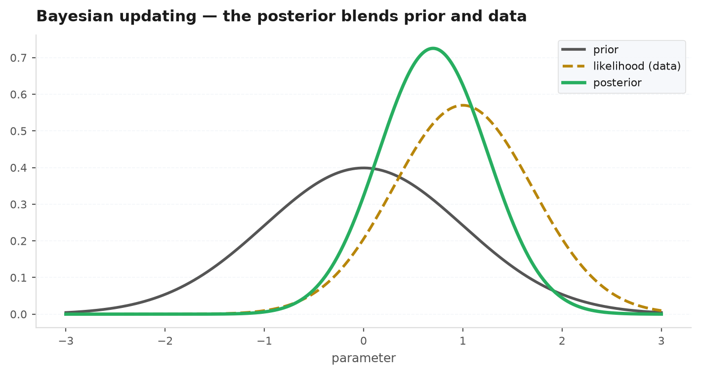
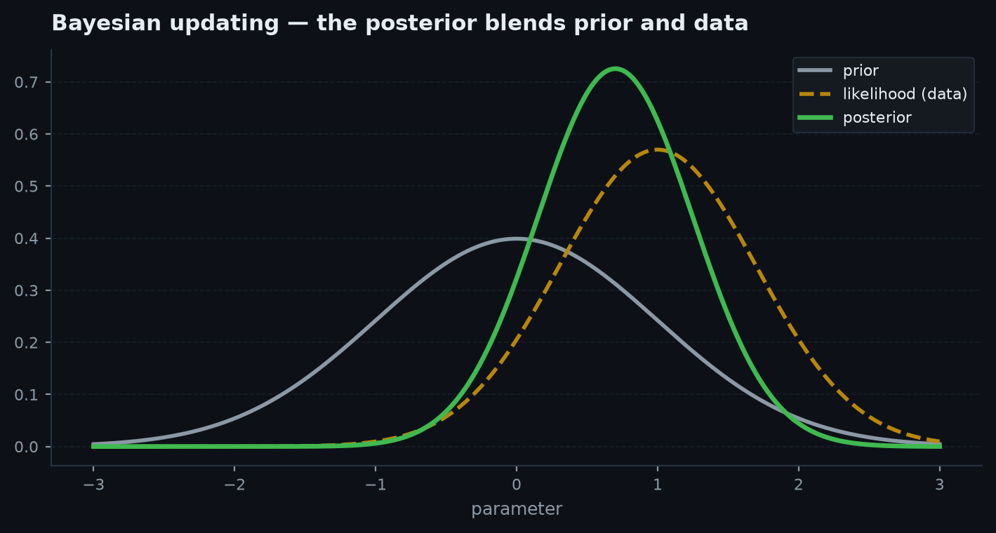
The cleanest case: estimate an unknown mean (say, the true per-trade edge) from Gaussian data with known variance . Put a Gaussian prior on centred at with variance . The magic of conjugacy is that the posterior is Gaussian too — the family is closed under updating, so we only need to track a mean and a variance.
It is cleanest in terms of precision = 1/variance. Prior precision ; each of observations carries precision . Multiply the Gaussian prior by the Gaussian likelihood of the sample mean and complete the square in . The exponent is
a quadratic in , so the posterior is Gaussian. Matching the quadratic and linear coefficients, the posterior precision is the sum of precisions and the posterior mean is the precision-weighted average of the two estimates:
Why it matters: the posterior mean is a weighted blend of your prior belief and the data’s estimate , with weights equal to how precisely each is known. With little data (small ) the prior dominates and your estimate stays near ; as the data precision swamps the prior and . Evidence overwhelms belief — but only in proportion to how much evidence you actually have. The posterior variance also shrinks monotonically, so more data always sharpens the estimate.
Win rate is a probability, not a mean, so the natural conjugate pair is Beta prior + Binomial likelihood. A density is proportional to ; the likelihood of wins in trades is proportional to . Multiply them and the exponents simply add — the posterior is , conjugacy in one line:
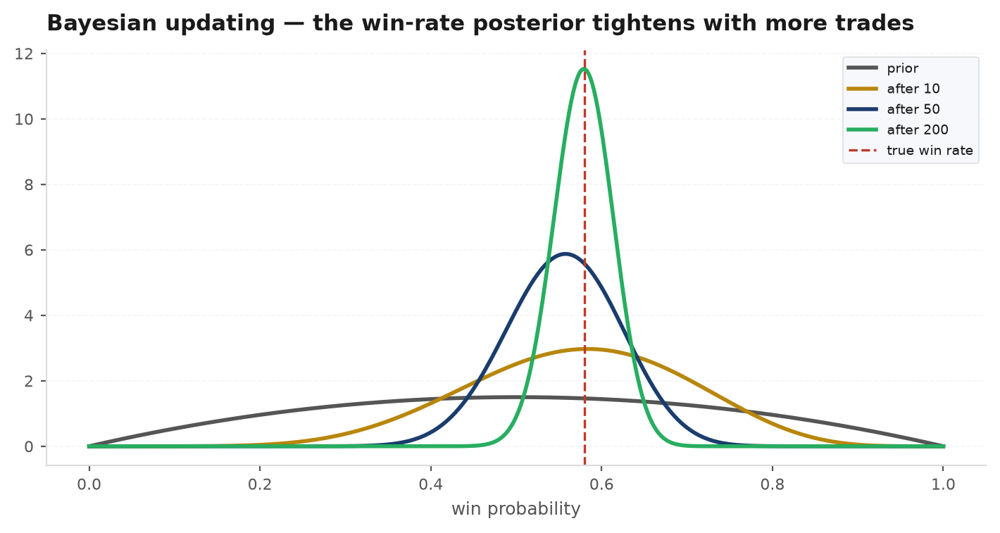
Put a weak, skeptical prior centred at a coin flip: (mean , worth just two pseudo-wins and two pseudo-losses). Observe wins and losses over trades. The posterior is , with
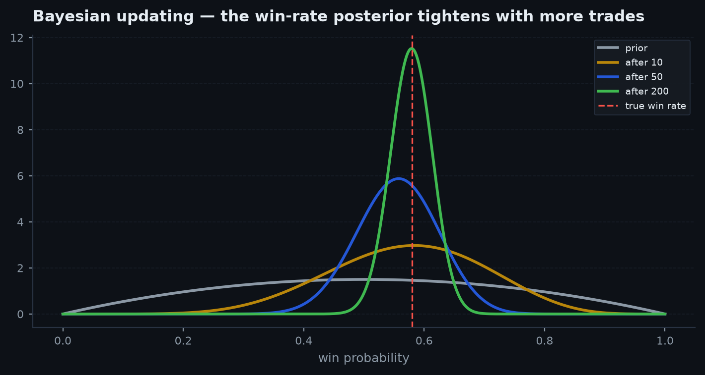
The raw sample win rate was ; the prior shrinks it to — barely, because 30 trades already outweigh a two-pseudo-trade prior. But look at the width: a 95% credible interval is roughly . If your payoff is the break-even win rate is , and sits comfortably insidethat interval. So the honest read after 30 trades is not “win rate, edge confirmed” but “probably above break-even, plausibly not — keep trading and let the posterior tighten.” That is the same “wide posterior = I don’t know yet” discipline as the Normal case, now on a bounded probability.
Credible vs confidence intervals#
The posterior lets you make the statement people think a confidence interval makes. A 95% credible interval is a range that contains the parameter with 95% posterior probability:
That is a direct probability statement about — exactly what you want. A frequentist confidence interval means something subtly but importantly different: 95% of intervals constructed this way across hypothetical repeat experiments would cover the true (fixed) . It says nothing about the probability that your particular interval contains it.
Shrinkage and regression to the mean#
The precision-weighted mean is shrinkage in disguise. Write it as the data estimate pulled a fraction of the way back toward the prior:
A noisy estimate from little data (small ) gets shrunk hard toward the prior; a well-measured one is left alone. This is the mathematics behind regression to the mean: extreme sample results are disproportionately lucky extremes, so the best forecast of the next sample is closer to the average than the last one was. It is also exactly the logic of Ledoit-Wolf covariance shrinkage from the optimization chapter — pull noisy estimates toward a stable target — and of fractional Kelly: since your edge is estimated, bet as if it were smaller than measured.
The base-rate reminder#
Bayes forces you to confront the base rate — the prior probability of a real edge — and it is low. Suppose 5% of the strategies you dream up have a genuine edge, and your validation test correctly flags a real edge 80% of the time but also fires on 10% of dead strategies (false positives). If a strategy passes, what is the chance it is real?
Even a good test, applied to a population that is mostly noise, leaves a passing strategy more likely dead than alive. The low base rate dominates. That is why edgekit’s gauntlet stacks multiple independent tests (permutation, walk-forward, regime split, cost stress): each one lowers the false-positive rate, and only their conjunction pushes the posterior probability of a real edge high enough to deploy.
Bayesian strategy allocation & Thompson sampling#
The Bayesian view also solves a live problem: you have several strategies and must decide how much to run each, while still learning which are best. That is the explore/exploit trade-off, and Thompson samplingis its elegant Bayesian solution. Keep a posterior over each strategy’s edge; to allocate, draw one sample from each posterior and back the strategy with the best draw.
- Exploit: strategies with high posterior means get chosen most often — you ride what is working.
- Explore: a strategy with few trades has a wide posterior, so its sample occasionally comes out on top — you keep giving uncertain strategies a chance, in exact proportion to how uncertain they are.
- Self-correcting: as evidence accumulates each posterior narrows, exploration automatically fades, and allocation converges on the genuinely best performers.
The allocation weight on a strategy is just the posterior probability that it is best, , estimated by the fraction of draws it wins. It needs no tuning parameter — the exploration rate is set by the posteriors themselves — which is why it beats hand-tuned -greedy rules in practice.
import numpy as np

# Posterior over each strategy's edge: mean m_k, std s_k (from the Normal update above).
# Thompson step: sample one edge per strategy, allocate to the argmax.
def thompson_weights(means, stds, draws=10_000, rng=np.random.default_rng(0)):
    samples = rng.normal(means, stds, size=(draws, len(means)))  # draws x K
    winners = samples.argmax(axis=1)                              # best draw each round
    return np.bincount(winners, minlength=len(means)) / draws     # P(strategy is best)

# Wide posterior (few trades) => more exploration; narrow => exploitation.
w = thompson_weights(means=[0.05, 0.02, 0.08], stds=[0.03, 0.03, 0.12])| Concept | Formula / rule | Trading use |
|---|---|---|
| Posterior | Belief about the edge after data | |
| Posterior mean | Shrunk edge estimate | |
| Credible interval | Honest range on the edge | |
| Shrinkage | Discount lucky backtests | |
| Thompson sampling | Explore/exploit allocation |
Next: you now have the full mathematical toolkit — linear algebra, regression, optimization, stochastic processes, and Bayesian inference. Take it back to the workbench and turn a raw idea into a validated strategy in Anatomy of a strategy.