Linear algebra for quants

A portfolio is a weighted sum of assets, and its risk is a quadratic form in those weights. Once you see that, the whole machinery of portfolio theory — variance, diversification, risk factors — collapses into three objects from linear algebra: a weight vector, a covariance matrix, and its eigenvectors. This chapter builds that vocabulary from the ground up, derives the one formula every optimizer uses, and shows why the eigenvectors of the covariance matrix arethe market’s hidden risk factors.

✦Intuition — before any symbols

Forget matrices for a second. You hold three things: some Bitcoin, some Ether, a little gold. Two questions run your book. What did I make today?— add up each holding’s move, weighted by how much of it you own. How risky am I? — that one is subtler, because BTC and ETH tend to crash together, so holding both is not two bets but nearly one, while gold usually zigs when crypto zags and quietly cancels risk. Linear algebra is just the bookkeeping that turns those two questions into a vector (the first) and a matrix sandwiched between two vectors (the second). Everything hard in this chapter is a way of reading that second object — the covariance matrix — correctly.

Vectors: returns and weights#

Take $N$ assets. On a given day their returns are just a list of numbers, which we stack into a column vector $r \in R^{N}$ . How you split your capital across them is a second vector, the weights $w \in R^{N}$ , where $w_{i}$ is the fraction of the book in asset $i$ . “Fully invested” is the linear constraint that the weights sum to one:

w^{⊤} 1 = i = 1 \sum N w_{i} = 1, 1 = (1, 1, \dots, 1)^{⊤} .

The portfolio’s return for the day is the dot productof the two — each asset’s return scaled by how much you held of it, summed:

r_{p} = w^{⊤} r = i = 1 \sum N w_{i} r_{i} .

The superscript $⊤$ is transpose: it turns the column $w$ on its side so the multiplication lines up term-by-term. Everything that follows is built by stacking these vectors into matrices and asking what happens to the dot products.

The covariance matrix Σ#

Return is linear in the weights, so its expectation is trivial: $E [r_{p}] = w^{⊤} μ$ where $μ = E [r]$ is the vector of expected returns. Risk is where the structure lives, because it depends on how assets move together. That co-movement is packed into the covariance matrix $Σ$ , an $N \times N$ table whose entries are

Σ_{ij} = Cov (r_{i}, r_{j}) = E [(r_{i} - μ_{i}) (r_{j} - μ_{j})] .

The diagonal $Σ_{ii} = Var (r_{i}) = σ_{i}^{2}$ is each asset’s own variance; the off-diagonal $Σ_{ij}$ is how asset $i$ and asset $j$ co-vary. Because $Cov (r_{i}, r_{j}) = Cov (r_{j}, r_{i})$ , the matrix is symmetric: $Σ = Σ^{⊤}$ . From a $T \times N$ matrix of historical returns $X$ (rows = periods, columns = assets), the sample estimate is a single matrix product on the demeaned data:

Σ^= \frac{1}{T - 1} X ~^{⊤} X ~, X ~ = X - X ˉ .

That is exactly what ek.optimize.sample_cov computes — a demeaned Gram matrix normalised by $T - 1$ . It is the maximum-likelihood covariance and it is the raw material for every risk calculation in the rest of Part VI.

cov.py

import edgekit as ek

# returns: T x N DataFrame (rows = days, columns = assets)
Sigma = ek.optimize.sample_cov(returns)   # N x N covariance, ddof=1
Sigma.shape          # (N, N)
Sigma.diagonal()     # per-asset variances (sigma_i^2)

Portfolio variance as a quadratic form#

Here is the formula that motivates the whole chapter. The variance of the portfolio return $r_{p} = w^{⊤} r$ is the quadratic form

σ_{p}^{2} = Var (w^{⊤} r) = w^{⊤} Σ w .

✦Derivation — expand the double sum, then collect it into a matrix product

Portfolio return is a weighted sum, $r_{p} = \sum_{i} w_{i} r_{i}$ . Variance of a sum expands into variances plus every pairwise covariance — this is the bilinearity of covariance, $Cov (\sum_{i} a_{i} X_{i}, \sum_{j} b_{j} Y_{j}) = \sum_{i, j} a_{i} b_{j} Cov (X_{i}, Y_{j})$ :

Var (i \sum w_{i} r_{i}) = i = 1 \sum N j = 1 \sum N w_{i} w_{j} Cov (r_{i}, r_{j}) = i, j \sum w_{i} w_{j} Σ_{ij} .

The right-hand double sum is, by the definition of matrix multiplication, precisely $w^{⊤} Σ w$ : multiplying $Σ$ by $w$ on the right forms the inner sum over $j$ , and the outer $w^{⊤}$ forms the sum over $i$ . Hence $σ_{p}^{2} = w^{⊤} Σ w$ . Why it matters: risk is not the weighted average of individual risks — the cross terms are the whole story. Two volatile assets with negative covariance can combine into a low-variance book; that cancellation, buried in the off-diagonals, is what diversification means mathematically.

Split the double sum into its diagonal and off-diagonal parts to read the diversification directly:

σ_{p}^{2} = own risk i \sum w_{i}^{2} σ_{i}^{2} + interaction i \neq = j \sum w_{i} w_{j} Σ_{ij} .

If the assets were uncorrelated the second term vanishes and risk is just the weighted sum of variances. Real assets are correlated, and the sign and size of that second term is what an optimizer is really trading against return. When correlations are positive it inflates risk; when some are negative it deflates it — the free lunch of diversification.

✦Scenario — a 3-asset book of BTC, ETH, and gold

Put real-ish annualised numbers on the desk. Volatilities: $σ_{BTC} = 0.60$ , $σ_{ETH} = 0.75$ , $σ_{gold} = 0.15$ . Correlations: $ρ_{BTC,ETH} = 0.80$ (crypto moves together), $ρ_{BTC,gold} = 0.10$ , $ρ_{ETH,gold} = 0.05$ . Each covariance is $Σ_{ij} = ρ_{ij} σ_{i} σ_{j}$ , so the matrix is

Σ = 0.360 0.360 0.009 0.360 0.5625 0.0056 0.009 0.0056 0.0225, w = (\frac{1}{3}, \frac{1}{3}, \frac{1}{3})^{⊤} .

Now evaluate the quadratic form. The diagonal (“own risk”) contributes $\frac{1}{9} (0.360 + 0.5625 + 0.0225) = 0.1050$ ; the off-diagonal (“interaction”) contributes $\frac{1}{9} \cdot 2 (0.360 + 0.009 + 0.0056) = 0.0832$ . Add them:

σ_{p}^{2} = w^{⊤} Σ w = 0.1050 + 0.0832 = 0.1882 ⟹ σ_{p} = 43.4%.

Read the numbers. A trader who ignoredcorrelation would guess the book’s risk was the weighted average of vols, $(0.60 + 0.75 + 0.15) /3 = 50%$ . If the assets were truly uncorrelated the diagonal alone would give $0.1050 = 32.4%$ . Reality — $43.4%$ — sits between: the $0.80$ BTC/ETH correlation is almost the entire interaction term (it alone adds $2 \times 0.360/9 = 0.080$ of variance), while gold’s near-zero correlations barely move it. That single off-diagonal cell is why “I hold BTC and ETH” is closer to one bet than two — and why the calm, uncorrelated gold sleeve is doing the real diversification work despite its tiny weight-share of the risk.

Positive semi-definiteness#

A variance can never be negative. Since $σ_{p}^{2} = w^{⊤} Σ w$ is a variance for any weights whatsoever, the covariance matrix must satisfy

w^{⊤} Σ w \geq 0 for all w \in R^{N} .

A symmetric matrix with this property is called positive semi-definite (PSD). It is not a technicality — it is a hard constraint that every valid covariance must obey, and it has three consequences you will keep meeting:

All eigenvalues are $\geq 0$ . A negative eigenvalue would let you build a portfolio with negative variance — impossible. (Strictly positive eigenvalues make $Σ$ positive definite and therefore invertible.)
The inverse can be unstable. A near-zero eigenvalue means $Σ$ is nearly singular, so $Σ^{- 1}$ (which the optimizers of the next chapter need) explodes. This is the numerical face of over-fitting a covariance from too little data.
Sample estimates can break PSD. When you have fewer observations than assets ( $T < N$ ), the sample covariance is rank-deficient — it has exact zero eigenvalues and is only semi-definite. That is one of several reasons shrinkage estimators exist.

→Why edgekit ridges the inverse

Because a noisy sample

Σ

can have eigenvalues so small that the inverse is nonsense, ek.optimize adds a tiny multiple of the identity (

Σ + ε I

) when the condition number blows up. That nudges every eigenvalue up by

ε

, restoring a stable, still-PSD matrix without moving a well-behaved one. The principled version of the same idea — Ledoit-Wolf shrinkage — is the subject of the next chapter.

The correlation matrix#

Covariance mixes co-movement with scale — a large $Σ_{ij}$ could just mean two volatile assets. To see the pure relationship, standardise each asset by its own volatility. The result is the correlation matrix $ρ$ :

ρ_{ij} = \frac{Σ _{ij}}{σ _{i} σ _{j}} = \frac{Cov ( r _{i} , r _{j} )}{σ _{i} σ _{j}} \in [- 1, 1] .

In matrix form, with $D = diag (σ_{1}, \dots, σ_{N})$ the diagonal matrix of volatilities, $ρ = D^{- 1} Σ D^{- 1}$ — a unit-diagonal, symmetric, still-PSD matrix. It is the right object to look at, because every entry is on the same $[- 1, 1]$ scale. In edgekit, ek.portfolio.correlation takes a dict of strategy R-streams and returns exactly this matrix — the diagnostic you use to check that the sleeves of a book are actually diversifying rather than secretly the same bet.

corr.py

import edgekit as ek

# books: {"orb": r_series, "sma": r_series, ...} of daily-R Series
rho = ek.portfolio.correlation(books)   # unit-diagonal correlation DataFrame
rho.loc["orb", "sma"]                   # pairwise correlation of two sleeves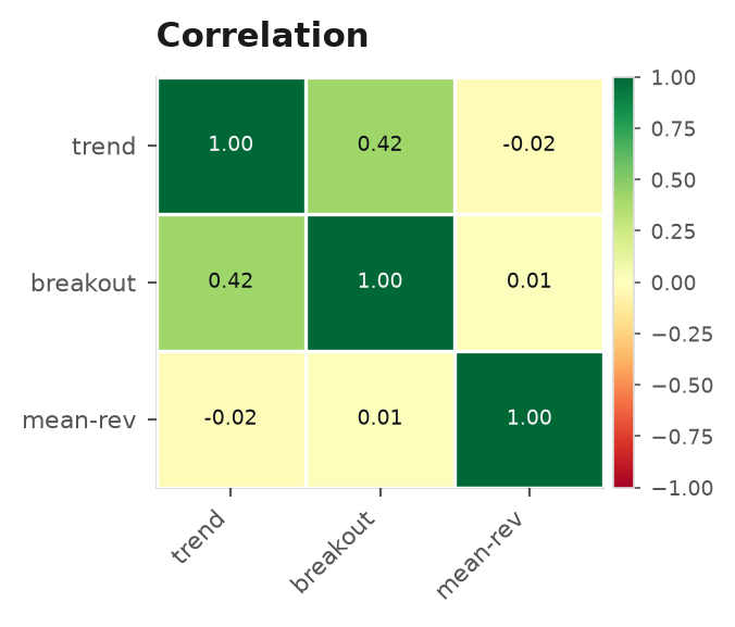

A heatmap of a correlation matrix, with a unit diagonal and colour-coded off-diagonal correlations — A correlation matrix as a heatmap. The unit diagonal is trivial; the off-diagonal block is what you read. Warm clusters are groups of assets that move together — a hint that the effective number of independent bets is smaller than the number of assets.

!A correlation heatmap hides the effective bet count

Eyeballing pairwise correlations tells you which assets look related, but not how many independent risks you truly hold. Ten assets that all correlate at 0.8 are close to one bet, not ten. Answering “how many bets do I really have?” needs the eigenvalues of the matrix — which is exactly what PCA delivers.

Eigenvalues, eigenvectors, and PCA#

A symmetric PSD matrix has a special structure: it can be written entirely in terms of its eigenvectors and eigenvalues. An eigenvector $v$ is a direction that $Σ$ merely stretches without rotating, and its eigenvalue $λ$ is the stretch factor:

Σ v = λ v .

The spectral theorem says any symmetric $Σ$ decomposes into an orthonormal set of $N$ such eigenvectors, collected as columns of an orthogonal matrix $V$ , with eigenvalues on a diagonal matrix $Λ$ :

Σ = V Λ V^{⊤} = k = 1 \sum N λ_{k} v_{k} v_{k}^{⊤}, λ_{1} \geq λ_{2} \geq \dots \geq λ_{N} \geq 0.

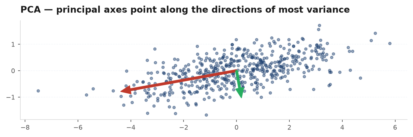
This is Principal Component Analysis. Each eigenvector $v_{k}$ — a principal component — is a specific combination of the assets (a synthetic portfolio), and its eigenvalue $λ_{k}$ is the variance of returns along that direction.

A 2D cloud of return points with two arrows from its centre along the principal-component directions, the longer arrow along the direction of greatest spread — Eigenvectors of the covariance, drawn on the data. The arrows point along the principal components — directions the matrix only stretches, not rotates — and each arrow's length is its eigenvalue, the variance along it. The long arrow is the highest-variance combination of the assets; the short one is what is left over and uncorrelated with it.

✦Derivation — the variance captured by a principal component is its eigenvalue

Consider the portfolio whose weights are a unit-length eigenvector, $w = v_{k}$ with $∥ v_{k} ∥ = 1$ . Its variance is the quadratic form from above; substitute the eigenvector equation $Σ v_{k} = λ_{k} v_{k}$ :

σ_{p}^{2} = v_{k}^{⊤} Σ v_{k} = v_{k}^{⊤} (λ_{k} v_{k}) = λ_{k} (v_{k}^{⊤} v_{k}) = λ_{k} .

So the variance of the return along principal component $k$ is exactly its eigenvalue. The largest eigenvalue $λ_{1}$ belongs to the highest-variance direction in the whole asset space — no unit-weight portfolio has more variance, which is a one-line consequence of the Rayleigh quotient $max_{∥ w ∥ = 1} w^{⊤} Σ w = λ_{1}$ . Because the eigenvectors are orthogonal, the components are uncorrelated synthetic assets, and the trace identity $\sum_{k} λ_{k} = tr (Σ) = \sum_{i} σ_{i}^{2}$ says the eigenvalues simply repartition the total variance of the market into independent buckets.

The fraction of total variance explained by the first $m$ components is the cumulative eigenvalue ratio, and it is the honest answer to “how many independent risks am I holding?”:

variance explained by top m = \frac{\sum _{k = 1}^{m} λ _{k}}{\sum _{k = 1}^{N} λ _{k}} .

A scree plot: variance explained by each principal component, with a steep drop after the first few and a cumulative curve — A PCA scree plot. The first component alone often captures most of the variance of a basket of correlated assets, and a handful more capture nearly all of it — the long tail of tiny eigenvalues is noise. The number of components needed to reach ~90% is the effective number of bets.

✦Scenario — how many bets are in the BTC/ETH/gold book?

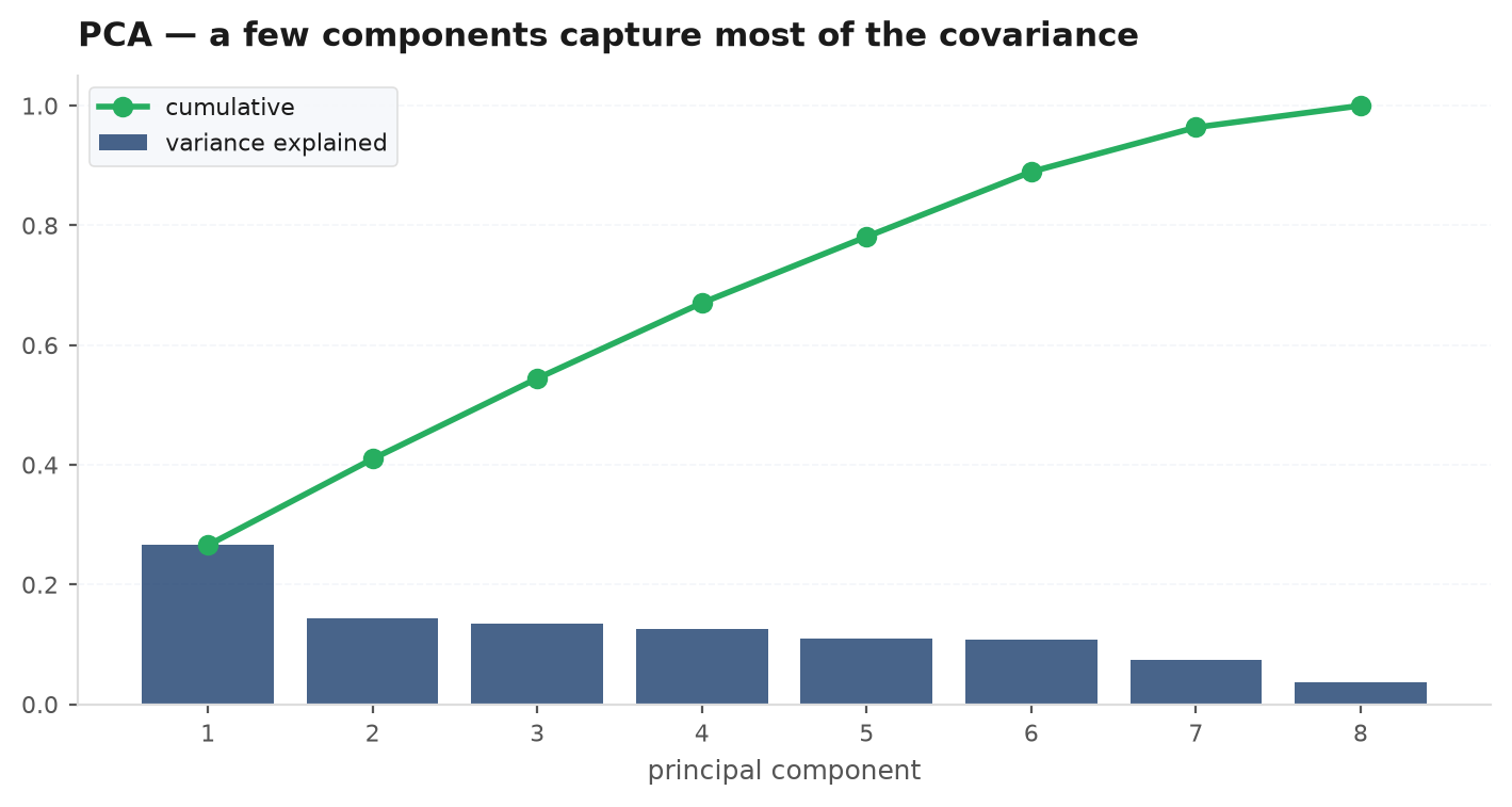
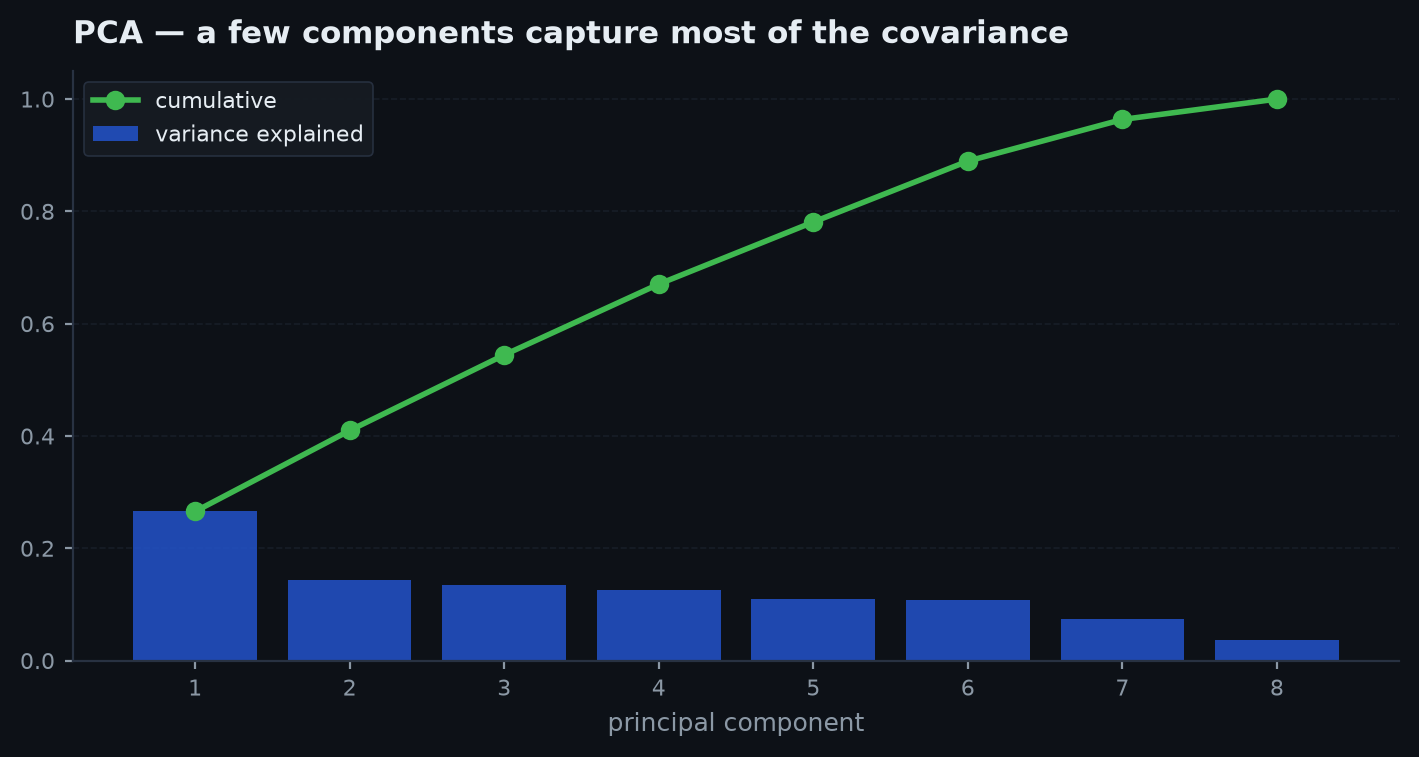
Diagonalise the $Σ$ from the scenario above and its three eigenvalues come out roughly $λ_{1} \approx 0.84$ , $λ_{2} \approx 0.087$ , $λ_{3} \approx 0.022$ (they sum to $tr (Σ) = 0.360 + 0.5625 + 0.0225 = 0.945$ , as the trace identity demands). The top eigenvector is almost entirelya long-BTC/long-ETH combination — that is “crypto beta,” and it alone is $0.84/0.945 = 89%$ of the total variance. The second eigenvector is dominated by gold. The upshot: three tickers, but $89%$ of your risk lives on one axis — you are running closer to one and a bitindependent bets, not three. That is the number a correlation heatmap cannot tell you but the eigenvalues can, and it is exactly what a risk manager means by “effective breadth.”

Why PCA finds risk factors#

The eigenvectors are not just a numerical convenience — for financial returns they line up with economically meaningful risk factors. When you run PCA on a basket of correlated assets you almost always see the same pattern:

The first component is “the market.” Its eigenvector has the same sign in every asset — a roughly equal-weight long that goes up when everything goes up. For equities it typically explains the large majority of the variance; it is the systematic beta that no amount of stock-picking diversifies away. This is the linear-algebra shadow of the market factor.
Later components are style/sector spreads. The second and third components have mixed signs — long one group, short another — and correspond to interpretable tilts (sector, size, value, duration). They are the market-neutral spreads a relative-value trader lives on.
The tail is noise. The many tiny eigenvalues correspond to idiosyncratic wiggle. A near-zero $λ$ is precisely the near-singular direction that destabilises $Σ^{- 1}$ — over-fitting risk, made visible.

This is why factor models and PCA are two views of the same object: a factor model $r = B f + ε$ says returns are driven by a few common factors $f$ , and PCA discovers those factors as the top eigenvectors of $Σ$ without being told what they are. The next chapter takes the complementary route: given a factor you name in advance (the market), regress against it to measure exposure.

Object	Symbol	Linear-algebra role	edgekit
Weights	$w$	Vector, sums to 1	portfolio weights
Covariance	$Σ$	Symmetric PSD matrix	ek.optimize.sample_cov
Correlation	$ρ$	Standardised Σ, unit diagonal	ek.portfolio.correlation
Portfolio variance	$w^{⊤} Σ w$	Quadratic form	ek.optimize.portfolio_vol
Risk factors	$v_{k}, λ_{k}$	Eigenvectors / eigenvalues of Σ	PCA (numpy.linalg.eigh)

→The one idea to keep

Risk is a quadratic form

w^{⊤} Σ w

; diversification is the cancellation in its off-diagonal terms; and the eigenvectors of

Σ

are the independent directions of that risk. Optimization (next chapter but one) is nothing more than minimising this quadratic form subject to linear constraints — which is where Lagrange multipliers enter.

Next: we have the covariance matrix and its factors — now we name a factor in advance and measure how much of a return it explains. Regression & factor models.