Optimization & portfolios

Given a covariance matrix and a set of return views, what weights should you hold? Markowitz turned that into a constrained optimization problem with a clean closed-form answer — and six decades of experience turned it into a cautionary tale about trusting your inputs. This chapter derives the minimum-variance and tangency portfolios with Lagrange multipliers, draws the efficient frontier, and then explains, honestly, why the elegant solution so often loses to naive 1/N out of sample.

✦Intuition — the shape of the problem

You have a pile of cash and a handful of assets. Put too much in the high-return one and a bad month wrecks you; spread it evenly and you leave return on the table. Somewhere between those extremes is a “best” split — and because risk is that bowl-shaped quadratic $w^{⊤} Σ w$ from the last chapter, there is exactly onebottom of the bowl, so “best” is well-defined and reachable by formula rather than by trial and error. The catch, which the second half of the chapter is honest about: the formula’s answer is only as good as the return and covariance estimates you feed it, and those are noisy. The whole arc is “here is the beautiful closed form; here is why the pros often trust a cruder, sturdier version of it.”

Convexity — why a unique answer exists#

Portfolio variance is the quadratic form $f (w) = w^{⊤} Σ w$ from Linear algebra for quants. Because $Σ$ is positive semi-definite, this function is convex: its Hessian is $\nabla^{2} f = 2Σ ⪰ 0$ , so the surface is a bowl with no false bottoms. That is what makes portfolio optimization tractable — a convex objective over linear constraints has a single global minimum, reachable in closed form. There is no local-minimum trap and no need for iterative solvers; the entire problem is one matrix inverse away.

Lagrange multipliers#

To minimise a function subject to equality constraints, we use Lagrange multipliers. The idea: at a constrained optimum, the gradient of the objective must be a linear combination of the constraint gradients — otherwise you could slide along the constraint surface and improve. Encode that by forming the Lagrangian, a single function whose stationary point solves the constrained problem. For “minimise $f (w)$ subject to $g (w) = 0$ ”:

L (w, λ) = f (w) - λ g (w), \nabla_{w} L = 0, \nabla_{λ} L = 0.

The second condition just re-imposes the constraint; the first is the stationarity condition. This single tool cracks both portfolios below.

The global minimum-variance portfolio#

The simplest Markowitz problem ignores returns entirely and asks for the least-risky fully-invested portfolio:

w min w^{⊤} Σ w subject to w^{⊤} 1 = 1.

✦Derivation — the closed-form min-variance weights

Form the Lagrangian with one multiplier for the budget constraint:

L (w, λ) = w^{⊤} Σ w - λ (w^{⊤} 1 - 1) .

Set the gradient in $w$ to zero, using $\nabla_{w} (w^{⊤} Σ w) = 2Σ w$ (valid because $Σ$ is symmetric):

\nabla_{w} L = 2Σ w - λ 1 = 0 ⟹ w = \frac{λ}{2} Σ^{- 1} 1 .

The weights are proportional to $Σ^{- 1} 1$ ; the multiplier $λ$ is just an overall scale, pinned by the budget constraint. Impose $w^{⊤} 1 = 1$ :

\frac{λ}{2} 1^{⊤} Σ^{- 1} 1 = 1 ⟹ \frac{λ}{2} = \frac{1}{1 ^{⊤} Σ ^{- 1} 1} .

Substitute back to get the celebrated closed form:

w_{mv} = \frac{Σ ^{- 1} 1}{1 ^{⊤} Σ ^{- 1} 1} .

Why it matters: notice the answer depends only on $Σ$ , never on expected returns. That is why min-variance is the most robust MVO output — there is no $μ$ to mis-estimate. On a diagonal $Σ$ it reduces to inverse-variance weighting, $w_{i} \propto 1/ σ_{i}^{2}$ — put more in the calm assets. The catch is the $Σ^{- 1}$ : it is exactly the noisy, near-singular inverse that the previous chapter warned about.

min_var.py

import edgekit as ek

Sigma = ek.optimize.sample_cov(returns)
w = ek.optimize.min_variance(Sigma)        # Sigma^{-1} 1 / (1' Sigma^{-1} 1)
w.sum()                                     # 1.0  (fully invested)
ek.optimize.portfolio_vol(w, Sigma)         # sqrt(w' Sigma w)

✦Scenario — the min-variance split of equities and gold by hand

Two assets make the closed form arithmetic you can do on paper. Take equities ( $σ_{1} = 16%$ , $μ_{1} = 8%$ ) and gold ( $σ_{2} = 15%$ , $μ_{2} = 4%$ ) with correlation $ρ = - 0.20$ , so $Σ_{12} = - 0.20 \times 0.16 \times 0.15 = - 0.0048$ . For two assets $w_{mv} = \frac{Σ ^{- 1} 1}{1 ^{⊤} Σ ^{- 1} 1}$ reduces to a one-liner:

w_{1} = \frac{σ _{2}^{2} - Σ _{12}}{σ _{1}^{2} + σ _{2}^{2} - 2 Σ _{12}} = \frac{0.0225 - ( - 0.0048 )}{0.0256 + 0.0225 - 2 ( - 0.0048 )} = \frac{0.0273}{0.0577} = 0.47.

So hold $47%$ equities, $53%$ gold. Plug back into the quadratic form:

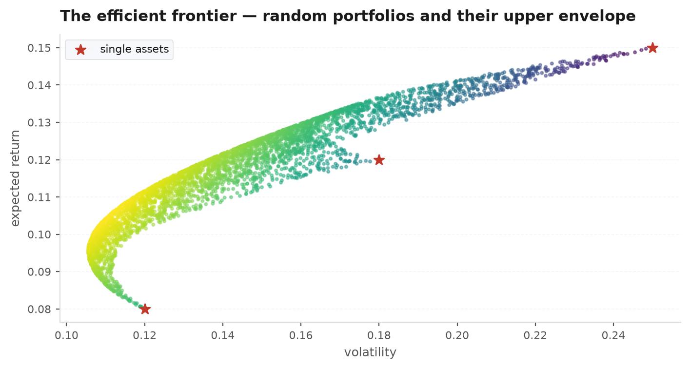
σ_{p}^{2} = 0.4 7^{2} (0.0256) + 0.5 3^{2} (0.0225) + 2 (0.47) (0.53) (- 0.0048) = 0.00959, σ_{p} = 9.8%.

Read that number: the least-risky asset alone had $15%$ vol, yet the blend sits at $9.8%$ — below either leg. That is the negative correlation cashing out as the diversification free lunch, and it is the leftmost nose of the efficient frontier drawn below. This min-variance mix earns $0.47 (8%) + 0.53 (4%) = 5.9%$ ; if you wanted more return you would slide right along the frontier, accepting more vol for it. Notice the whole calculation never touched expected returns until the very last line — which is why the min-variance point is the one Markowitz output you can trust when you distrust $μ$ .

→Unconstrained means shorts are allowed

The closed form places no sign restriction on

w

, so a weight can come out negative — a short position — whenever assets are strongly correlated. edgekit’s min_variance/max_sharpe are deliberately unconstrained; add your own box or no-short constraints downstream if the venue forbids shorting.

Adding a return target: the efficient frontier#

Now bring returns back. Minimise variance for a chosen target return $m$ , giving two constraints:

w min w^{⊤} Σ w s.t. w^{⊤} 1 = 1, w^{⊤} μ = m .

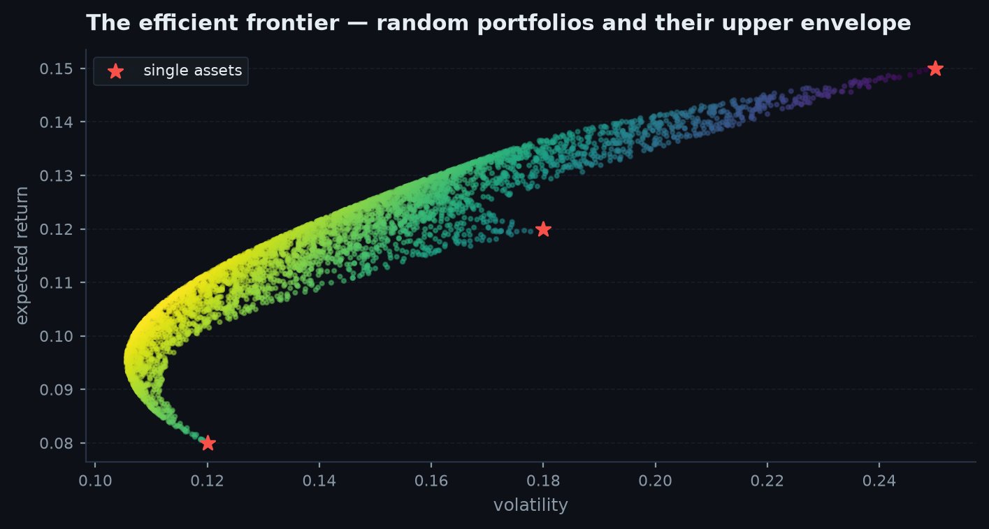
Two constraints means two multipliers. The stationarity condition $2Σ w = λ 1 + γ μ$ gives $w = \frac{1}{2} Σ^{- 1} (λ 1 + γ μ)$ , and solving the two constraints for $λ, γ$ makes the optimal weights affine in the target return — the two-fund theorem: $w (m) = g + h m$ . Sweeping $m$ traces a parabola in variance, whose upper branch is the efficient frontier: the set of portfolios with the highest return for each level of risk. edgekit computes the whole curve analytically (no per-point solve) with the constants $A = 1^{⊤} Σ^{- 1} 1$ , $B = 1^{⊤} Σ^{- 1} μ$ , $C = μ^{⊤} Σ^{- 1} μ$ :

σ^{2} (m) = \frac{A m ^{2} - 2 B m + C}{A C - B ^{2}} .

The efficient frontier: a curve of portfolio return against volatility, with individual assets inside it, the minimum-variance point at the far left, and the tangency portfolio where a line from the risk-free rate touches the curve — The efficient frontier. Every individual asset sits inside the curve; combining them pushes the achievable set up and to the left — that leftward shift is diversification. The nose of the curve is the global minimum-variance portfolio; the point where a line from the risk-free rate is tangent to the curve is the max-Sharpe (tangency) portfolio.

The tangency (max-Sharpe) portfolio#

Among all frontier portfolios, one has the steepest reward-per-risk — the highest Sharpe ratio $(w^{⊤} μ - r_{f}) / w^{⊤} Σ w$ . It is where a line drawn from the risk-free rate is tangent to the frontier, hence the tangency portfolio. Maximising the Sharpe ratio and solving gives another clean closed form:

w_{tan} \propto Σ^{- 1} (μ - r_{f} 1), normalised so w^{⊤} 1 = 1.

Under the two-fund theorem, every investor holds some mix of the risk-free asset and this one risky portfolio — risk preference only sets the split, not the composition. edgekit exposes it as ek.optimize.max_sharpe, and the full frontier (returns, vols, weights, Sharpe at each point) as ek.optimize.efficient_frontier.

frontier.py

import edgekit as ek

Sigma = ek.optimize.sample_cov(returns)
mu = returns.mean().to_numpy()             # expected-return VIEW (treat skeptically!)

w_tan = ek.optimize.max_sharpe(mu, Sigma, rf=0.0)   # Sigma^{-1}(mu - rf) normalised
front = ek.optimize.efficient_frontier(mu, Sigma, n=50)
front["vols"], front["returns"]            # trace the curve
front["sharpe"].max()                      # best reward-per-risk on the frontier

!max_sharpe is dangerously sensitive to μ

The tangency weights depend on

Σ^{- 1} μ

, and

μ

— expected returns — is the single hardest thing to estimate in finance. Small errors in

μ

get amplified by

Σ^{- 1}

into wildly concentrated, often heavily-short weights. The min-variance portfolio avoids this by dropping

μ

entirely; that is why it generalises better.

!Scenario — how a 0.5% estimate wobble flips the tangency book

Take two near-twin assets: $σ_{1} = σ_{2} = 20%$ , correlation $ρ = 0.90$ , and estimated returns $μ_{1} = 8%$ , $μ_{2} = 7%$ ( $r_{f} = 0$ ). The high correlation makes $Σ$ nearly singular, so $Σ^{- 1}$ is huge, and $w_{tan} \propto Σ^{- 1} (μ - r_{f} 1)$ comes out

w = (1.13, - 0.13) — 113% long asset 1, 13% short asset 2.

A $1%$ return gap became a leveraged long/short. Now nudge just one input — $μ_{2}$ from $7%$ to $7.5%$ , well within any estimation error — and the weights swing to $w = (0.81, 0.19)$ : the short flips to a fifth of the book long. Nothing about the world changed; a rounding error in $μ$ did, and $Σ^{- 1}$ amplified it into a different portfolio. That is the error-maximiser in one example — and the concrete reason the desk reaches for shrinkage, risk parity, or plain 1/N below.

Why the optimizer is fragile#

Markowitz optimization is an error-maximiser. It seeks out assets that look high-return and low-correlation — and those are precisely the estimates most likely to be lucky sampling noise. The inverse $Σ^{- 1}$ makes it worse: near-zero eigenvalues (see the PCA discussion) blow up into enormous long/short bets on directions that are pure estimation error. The result is a portfolio that is beautifully optimal in-sample and unstable out of sample.

Ledoit-Wolf shrinkage#

The standard fix is to shrink the noisy sample covariance toward a stable, structured target — a scaled identity $μ I$ ( $μ$ = average sample variance). Ledoit-Wolf picks the convex mix that minimises expected squared error, with the shrinkage intensity $δ$ available in closed form — no cross-validation:

Σ^{*} = δ μ I + (1 - δ) S, δ \in [0, 1] .

Shrinkage pulls the tiny, noise-dominated eigenvalues up and the inflated ones down — it conditions the matrix, so $(Σ^{*})^{- 1}$ stops exploding. The sample cov is unbiased but high-variance; the identity target is biased but stable; the convex blend trades a little bias for a large variance reduction. Because it is a mix of two PSD matrices it is itself PSD, and strictly better-conditioned than $S$ . Feed $Σ^{*}$ to the optimizers whenever the raw inverse looks unstable.

shrinkage.py

import edgekit as ek

S   = ek.optimize.sample_cov(returns)      # unbiased but noisy
Sig = ek.optimize.ledoit_wolf(returns)     # shrunk toward scaled identity — stable inverse

w_raw    = ek.optimize.min_variance(S)     # can be wild / heavily short
w_shrunk = ek.optimize.min_variance(Sig)   # tamer, more diversified weights

Risk parity — sizing by risk, not dollars#

A robust middle ground drops expected returns and the fragile inverse. Equal-risk contribution (risk parity) asks that every asset supply the same share of total portfolio variance. Using the Euler decomposition of the variance, asset $i$ ’s risk contribution is $RC_{i} = w_{i} (Σ w)_{i}$ , and these sum exactly to $w^{⊤} Σ w$ . Risk parity solves for the long-only $w$ where all $RC_{i}$ are equal — no single asset can dominate the risk budget. edgekit finds it with a stable damped fixed point (no matrix inverse at all):

erc.py

import edgekit as ek

Sigma = ek.optimize.sample_cov(returns)
w_erc = ek.optimize.equal_risk_contribution(Sigma)   # every asset = 1/N of the variance
ek.optimize.risk_contributions(w_erc, Sigma)         # ~equal entries, sum to portfolio variance

Why 1/N often wins out of sample#

Here is the humbling result. In a well-known study, DeMiguel, Garlappi & Uppal (2009) found that across many datasets, sophisticated mean-variance optimizers failed to reliably beat the naive equal-weight (1/N) portfolio out of sample. The reason is exactly the fragility above: the estimation error in $μ$ and $Σ$ costs more than the theoretical optimization gain. Equal weighting has zero estimation error — there are no parameters to get wrong.

Method	Uses μ?	Uses Σ⁻¹?	Estimation risk	edgekit
1/N equal weight	No	No	None	(w = 1/N)
Risk parity (ERC)	No	No (fixed point)	Low	equal_risk_contribution
Min-variance	No	Yes	Medium	min_variance
Min-variance + shrinkage	No	Yes (conditioned)	Lower	ledoit_wolf → min_variance
Max-Sharpe (tangency)	Yes	Yes	High	max_sharpe

✦The practical hierarchy

The more an allocator relies on estimated inputs, the more it over-fits. So the robust ordering runsup the table: prefer 1/N or risk parity, reach for min-variance only with shrinkage, and treat max-Sharpe as a fragile view that needs strong priors on

μ

. This is precisely why edgekit’s deployment-facing portfolio construction layer combines validated R-streams with inverse-vol and hierarchical risk parity by default, keeping the fragile matrix inverse out of the live sizing path.

The lesson is not that optimization is useless — it is that its inputs must be defensible. Use it when you have few assets, a long history, and a shrunk covariance you trust; fall back to risk-based heuristics when you do not. The math gives you the optimum conditional on the inputs being right; the discipline is knowing how wrong the inputs are.

Next: we have modelled portfolios of returns — now we model how a single price moves through time, the random process the whole edifice rests on. Stochastic processes.