Information theory for traders

An edge is information the market has not priced. Information theory makes that sentence literal: it measures information in bits, gives a dependence measure that catches what correlation misses, and — through a result that still feels like a magic trick — shows that the growth rate of optimally-bet capital equals the information rate of your signal. Kelly sizing is not merely related to information theory; it is information theory, with wealth as the channel decoder.

✦Intuition — why bits are the right unit for edge

Suppose someone whispers tomorrow’s direction to you and is right 100% of the time. Each whisper resolves one fair coin — one bit — and with even-money bets you can double your capital every day: one bit in, one doubling out. Now degrade the whisperer to 55% accuracy. The whisper still carries information, but much less than a bit — and, correspondingly, your best possible compound growth collapses from one doubling per bet to a small fraction of one. That exchange rate — bits of information in, doublings of capital out — is exact, not a metaphor, and it is the cleanest way to understand why real edges (a few hundredths of a bit) take hundreds of bets to compound into anything, and why anyone claiming to double monthly is claiming an information channel no market leaves open.

Entropy: the size of your uncertainty#

Start with a discrete random variable $X$ taking values with probabilities $p_{i}$ . Its Shannon entropy is

H (X) = - i \sum p_{i} lo g_{2} p_{i} bits .

Entropy is the average surprise: $- lo g_{2} p_{i}$ is how surprising outcome $i$ is (rare events carry more surprise), and $H$ averages it over the distribution. A fair coin has $H = 1$ bit — maximal uncertainty for two outcomes. A biased coin with $p = 0.55$ has

H (0.55) = - 0.55 lo g_{2} 0.55 - 0.45 lo g_{2} 0.45 \approx 0.9928 bits,

barely below the maximum — which already tells you a 55/45 edge is a whisper, not a shout. For market returns, entropy measures how unpredictable the return stream is: a perfectly efficient market maximises the entropy of the sign of the next return given the past. Rolling entropy of binned returns is therefore a crude efficiency gauge — entropy dropping below its usual level flags a window where returns became more structured (trending, stuck at a peg, regime-bound), which is precisely when simple rules start working.

rolling_entropy.py

import edgekit as ek

# Rolling Shannon entropy of binned returns: a crude market-efficiency gauge.
# High entropy ~ returns look like fair coin flips; dips ~ structure crept in.
r = bars["close"].pct_change().dropna()
ent = ek.timeseries.shannon_entropy(r, bins=10, window=100)   # pd.Series, bits
ent.tail()

KL divergence: the cost of a wrong model#

The Kullback-Leibler divergence measures how far a distribution $q$ (your model) is from the truth $p$ :

D_{KL} (p ∥ q) = i \sum p_{i} lo g_{2} \frac{p _{i}}{q _{i}} \geq 0, = 0 ⟺ p = q .

Read it as the number of extra bits you pay, per observation, for coding reality with the wrong model. It is asymmetric — being wrong about tails costs differently than being wrong about the centre — and it is the natural loss behind maximum likelihood: fitting by ML is minimising the KL divergence from the empirical distribution to your model. For a trader the sharpest reading is this: your compound growth deficit from betting with the wrong probabilities is a KL divergence. If reality deals outcomes from $p$ but you size positions as if they came from $q$ , your Kelly growth rate falls short of the optimum by exactly $D_{KL} (p ∥ q)$ bits per bet. Model error is not an abstraction — it has a price, denominated in doublings.

Mutual information: dependence beyond correlation#

Correlation measures linear co-movement. Mutual information measures dependence of any shape. For two variables it is the KL divergence between their joint distribution and the product of their marginals — how far reality is from independence:

I (X; Y) = D_{KL} (p (x, y) ∥ p (x) p (y)) = H (X) - H (X ∣ Y) .

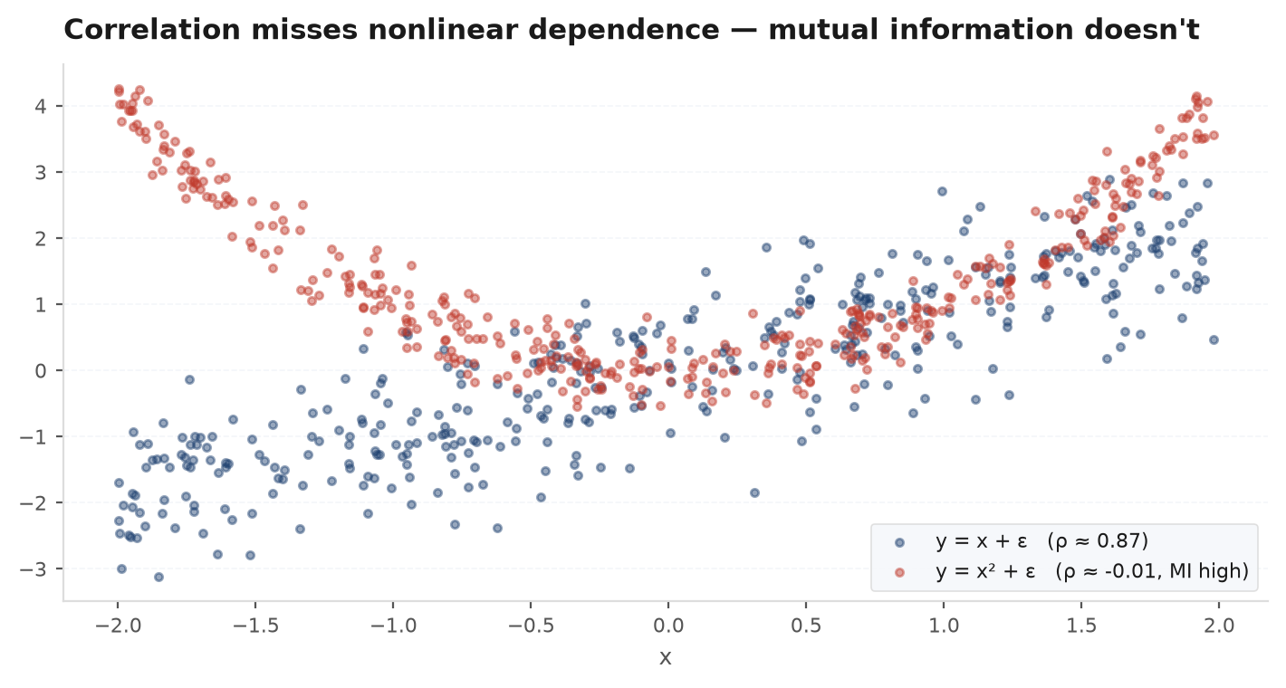
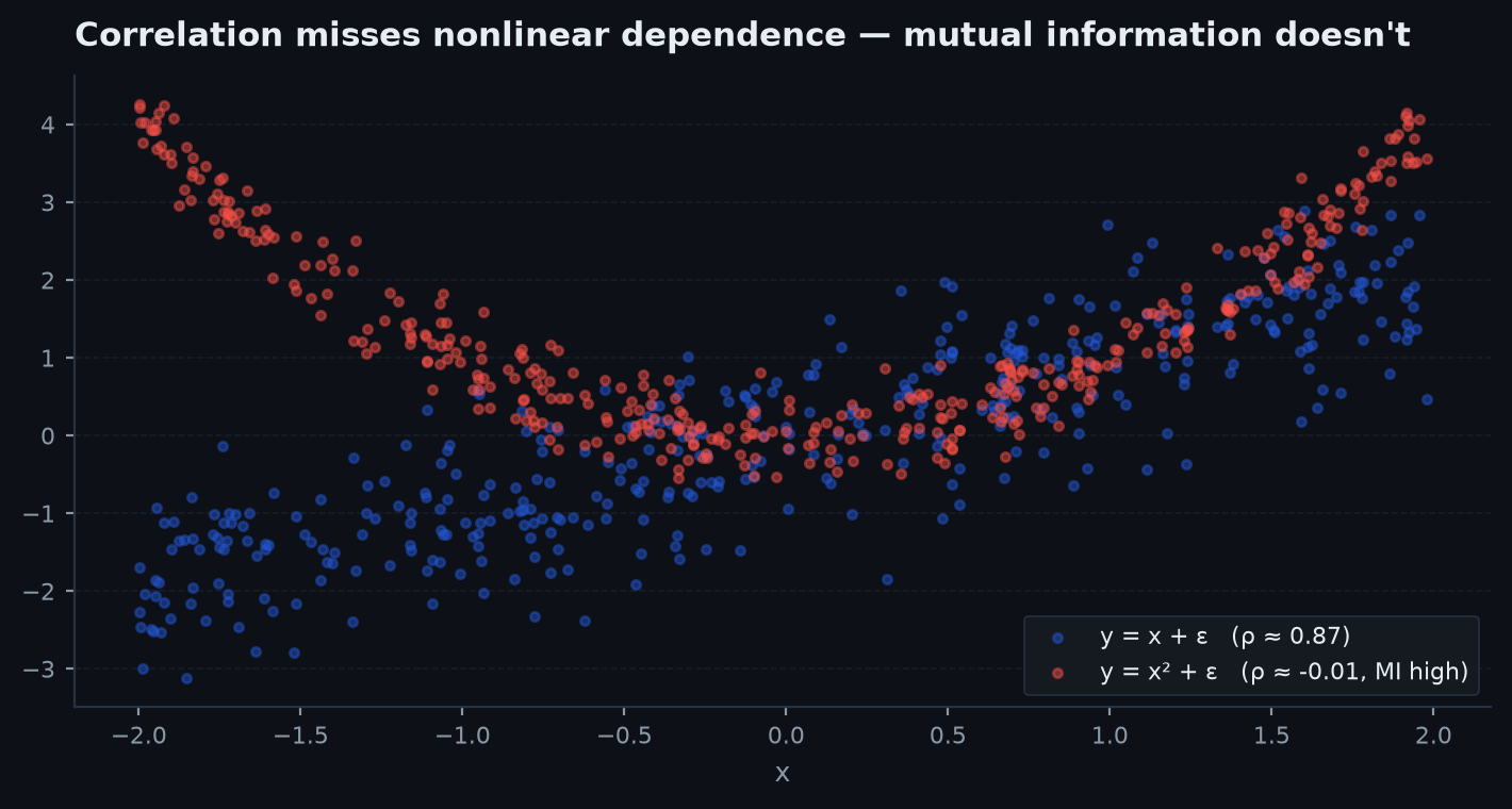
The second form is the operational one: mutual information is how many bits of uncertainty about $X$ are removed by observing $Y$ . It is zero if and only if the variables are independent — a much stronger statement than zero correlation. The canonical counterexample: let $Y = X^{2}$ with $X$ symmetric around zero. Correlation is exactly zero (the relationship has no linear part), yet $Y$ is a deterministic function of $X$ — mutual information is maximal. Volatility signals live in exactly this blind spot: the magnitudeof yesterday’s return predicts the magnitude of today’s (volatility clustering) while the signed correlation stays near zero. Correlation says markets are unpredictable; mutual information says their risk is highly predictable. Both are right.

Scatter plots of relationships with near-zero correlation but high mutual information, such as a quadratic and a volatility-clustering pattern, contrasted with a linear relationship — Correlation vs mutual information. Left: a linear relationship — both measures detect it. Right: a symmetric nonlinear dependence (returns vs squared returns, the shape of volatility clustering) — correlation is ~0 while mutual information is large. MI is zero only under true independence; correlation is zero under mere linear independence.

→For Gaussians, MI and correlation agree — that is the special case

(X, Y)

are jointly Gaussian with correlation

ρ

, mutual information collapses to

I = - \frac{1}{2} lo g_{2} (1 - ρ^{2})

— a monotone function of

∣ ρ ∣

, so the two rankings coincide. Every gap between MI and correlation is therefore a measure of non-Gaussian, nonlinear structure — which, per Part II, is where markets actually live.

mutual_info.py

import numpy as np

def mutual_information(x, y, bins=16):
    """Plug-in MI estimate (bits) from a 2-D histogram."""
    joint, _, _ = np.histogram2d(x, y, bins=bins)
    pxy = joint / joint.sum()
    px, py = pxy.sum(axis=1), pxy.sum(axis=0)
    nz = pxy > 0
    return float((pxy[nz] * np.log2(pxy[nz] / np.outer(px, py)[nz])).sum())

r = bars["close"].pct_change().dropna().to_numpy()
corr = np.corrcoef(r[:-1], np.abs(r[1:]))[0, 1]       # ~ 0: no linear link
mi   = mutual_information(r[:-1], np.abs(r[1:]))       # > 0: vol clustering

The information coefficient, in bits#

Practitioners score forecasting signals with the information coefficient (IC) — the correlation between forecast and subsequent return. A monthly IC of 0.05 is respectable; 0.10 is excellent. Information theory tells you how little that is in absolute terms. Using the Gaussian bridge above, an IC of $ρ = 0.05$ carries

I = - \frac{1}{2} lo g_{2} (1 - 0.0 5^{2}) \approx 0.0018 bits per forecast.

Two thousandths of a bit. That is the honest size of a good quant signal — and it is why the fundamental law of active management says value comes from breadth: many small, independent applications of a tiny edge. Information from independent signals adds; $n$ independent forecasts at IC $ρ$ deliver roughly $n$ times the bits, which is the information-theoretic reading of the $IR \approx IC n$ rule from The math of edge.

Kelly as channel capacity#

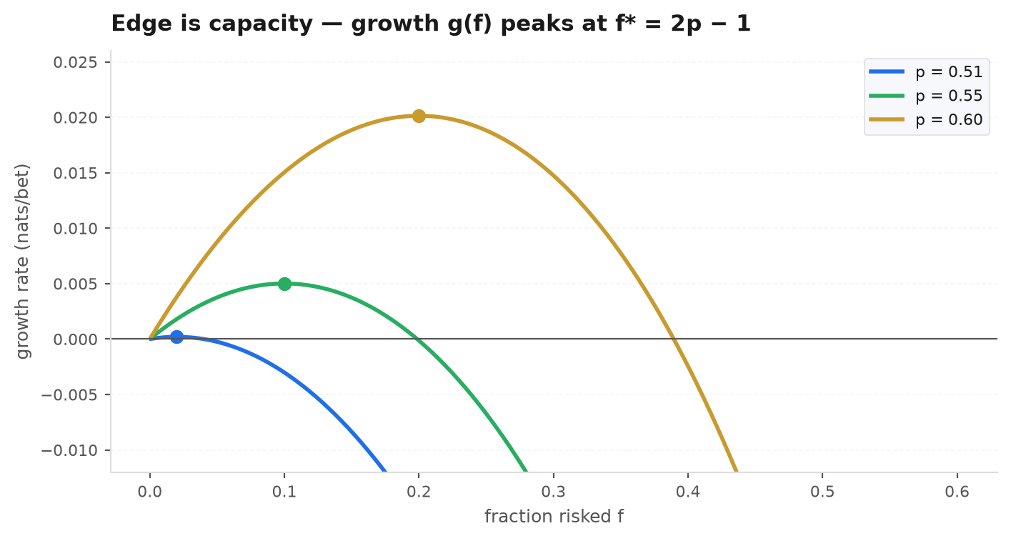
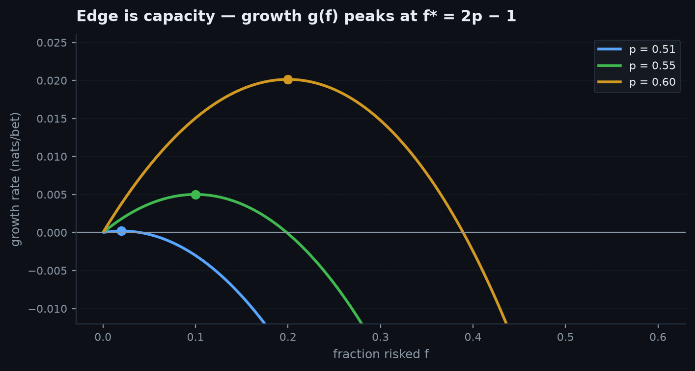
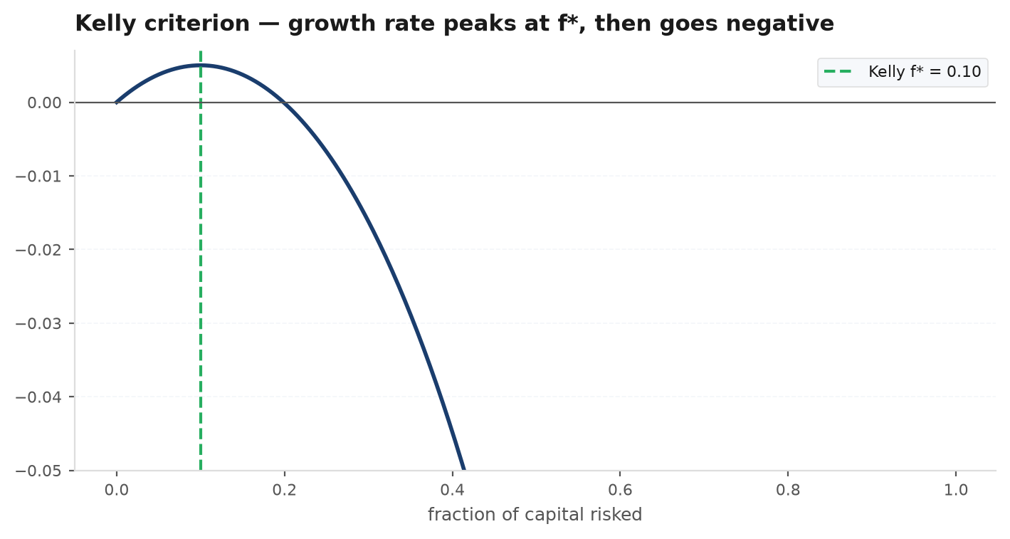
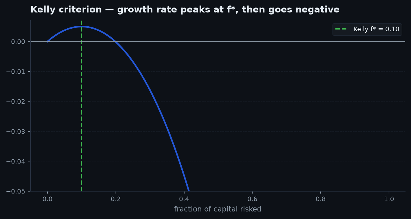
Now the centrepiece. Kelly showed (1956, at Bell Labs, in Shannon’s hallway) that for a repeated even-money bet won with probability $p > \frac{1}{2}$ , betting the fixed fraction $f^{*} = 2 p - 1$ of capital maximises the long-run growth rate, and the maximised growth is

G^{*} = 1 - H (p) = 1 + p lo g_{2} p + (1 - p) lo g_{2} (1 - p) doublings per bet.

✦Derivation — growth rate of fractional betting, then maximise

Bet a fraction $f$ each round. After $W$ wins and $L$ losses in $n = W + L$ rounds, capital is $V_{n} = V_{0} (1 + f)^{W} (1 - f)^{L}$ . The per-bet log growth is

G (f) = \frac{1}{n} lo g_{2} \frac{V _{n}}{V _{0}} n \to \infty p lo g_{2} (1 + f) + (1 - p) lo g_{2} (1 - f)

by the law of large numbers. Set the derivative to zero: $\frac{p}{1 + f} = \frac{1 - p}{1 - f}$ , giving $f^{*} = 2 p - 1$ . Substitute back with $1 + f^{*} = 2 p$ and $1 - f^{*} = 2 (1 - p)$ :

G^{*} = p lo g_{2} (2 p) + (1 - p) lo g_{2} (2 (1 - p)) = 1 - H (p) .

Why it matters: $1 - H (p)$ is exactly the capacity of a binary symmetric channel with error rate $1 - p$ — the maximum rate at which information can pass through a noisy wire that flips bits with probability $1 - p$ . Your forecast is the wire; the market outcome is the received symbol; your bankroll is the decoder. Optimally-bet capital grows at precisely the rate information arrives. Edge is measured in bits, and Kelly converts bits to wealth at par.

Growth rate of optimally bet capital as a function of win probability, tracing the channel capacity curve 1 minus binary entropy, zero at p equals one half and one bit at p equals one — Kelly growth equals channel capacity: G* = 1 − H(p), in doublings per bet. At p = 0.5 the channel is pure noise and the optimal bet — and growth — is zero. At p = 1 the channel is perfect: one bit per bet, capital doubles every round. Real edges live in the flat left corner of this curve.

✦Scenario — how many bits is a 55/45 edge, and how long to double?

You have a genuine 55/45 binary edge at even money — a strong signal by trading standards. Kelly says bet $f^{*} = 2 (0.55) - 1 = 10%$ of capital per trade. The information rate is

G^{*} = 1 - H (0.55) \approx 1 - 0.9928 = 0.0072 bits per bet.

Seven thousandths of a doubling per bet. Doubling your capital takes $1/0.0072 \approx 138$ bets — at one trade a day, about seven months of full-Kelly betting, enduring the drawdowns full Kelly implies (see Position sizingfor why half-Kelly, at ~three-quarters of the growth with far less pain, is the practitioner’s choice). The lesson cuts both ways. Downward: even a strong edge compounds slowly, because 55/45 carries almost no information. Upward: anyone who reliably doubles in weeks is implicitly claiming multiple bits per day — the informational equivalent of near-perfect foresight — which is how information theory lets you price the plausibility of a track record before seeing a single trade.

Long-run growth rate versus bet fraction for a favourable bet, peaking at the Kelly fraction and going negative beyond twice Kelly — The growth curve G(f) for the 55/45 bet. It peaks at f* = 0.10 (where growth equals the 0.0072-bit information rate), falls away on both sides, and crosses zero at 2f*: betting more than twice Kelly turns a winning edge into a losing strategy. Overbetting destroys information.

What the identities buy you at the desk#

A speed limit.Growth cannot exceed the information rate of your signals. Estimate the bits (via IC or MI) and you have a hard ceiling on believable performance — yours or a vendor’s.
A model-error tax. Betting with probabilities $q$ when truth is $p$ costs $D_{KL} (p ∥ q)$ bits per bet — the direct link between calibration (Part V) and compounding.
A better dependence screen. Mutual information catches nonlinear links — vol clustering, threshold effects, tail co-movement — that a correlation matrix scores as zero.
A reason for breadth. Bits from independent signals add. Ten independent 0.002-bit signals equal one 0.02-bit signal — and are far easier to find.

The theory assumes	Reality	Consequence
Known, stationary p	Edges are estimated and decay	Full Kelly on an estimated p overbets; shade down
Independent bets	Positions correlate; regimes cluster losses	Effective breadth (and bits) lower than count
Even-money binary payoffs	Continuous, skewed, fat-tailed P&L	Use the general Kelly (mu/sigma^2 form) with care
MI estimable from data	Histogram MI is biased upward in small samples	Compare against a shuffled-data null before believing it

!Estimated bits are not bits

Every quantity in this chapter is a property of the true distribution, which you never observe. A histogram MI on 500 observations will read positive on pure noise (finite-sample bias); an IC of 0.05 has a standard error that can swallow it whole; and full Kelly sized on an optimistically estimated

p

is over-betting — which the growth curve punishes asymmetrically. The gauntlet applies to information estimates exactly as it applies to backtests: test them against a shuffled null (Monte-Carlo methods) before spending their bits.

Next: the cleanest machine for extracting a small signal from noisy observations, one Bayesian update at a time — Kalman filters & state-space models.