Kalman filters & state-space models

Most quantities a trader cares about — the fair value under the noise, the current hedge ratio, the drift of a trend — are hidden states: you never observe them, only noisy measurements of them. State-space models make the hidden thing explicit, and the Kalman filter is the exact Bayesian machine for tracking it: every new observation updates your belief by a fraction of the surprise, with the fraction set by how much you trust your model versus your data. It is Bayesian updating, industrialised.

✦Intuition — a moving average that knows what it is doing

A moving average smooths a noisy price by averaging a window. But it makes two arbitrary choices: every point in the window counts equally, and everything before it counts for nothing. The Kalman filter replaces both with an answer derived from a model. If you tell it “the true level drifts a little each bar (process noise), and my observation of it is fuzzy (measurement noise),” it derives the optimal weighting — an exponential decay whose speed is not a parameter you tune but a consequence of the two noise levels. Better: it carries an error bar on its own estimate, and it updates in one line per bar. The same machinery that took Apollo to the moon tracks your hedge ratio; the only difference is the state you ask it to follow.

State-space form#

A (linear, Gaussian) state-space model is a pair of equations. The state equation says how the hidden state $x_{t}$ evolves; the observation equation says how the data $y_{t}$ you actually see is generated from it:

x_{t} = A x_{t - 1} + w_{t}, w_{t} \sim N (0, Q) (state / transition)

y_{t} = H x_{t} + v_{t}, v_{t} \sim N (0, R) (observation / measurement)

$Q$ is the process noise — how fast the hidden truth wanders — and $R$ is the measurement noise— how fuzzy each observation is. Their ratio is the model’s single most important quantity, as we will see. The framework is deceptively general: AR processes, hidden Markov regime models, time-varying regressions, and structural trend/cycle decompositions are all state-space models with different choices of $A$ , $H$ , $Q$ , $R$ . The simplest useful member is the local level model: $A = H = 1$ , so the true level is a random walk and you observe it plus noise.

Predict, then update#

The Kalman filter tracks the posterior of the state — a Gaussian, fully described by a mean $x^_{t}$ and a variance $P_{t}$ — with a two-step cycle each bar. For the local level model:

Predict:push yesterday’s belief through the state equation. The mean is unchanged (a random walk’s best forecast is its current value); the uncertainty grows by the process noise: $x^_{t ∣ t - 1} = x^_{t - 1}$ , $P_{t ∣ t - 1} = P_{t - 1} + Q$ .
Update: observe $y_{t}$ , compute the surprise (the innovation $y_{t} - x^_{t ∣ t - 1}$ ), and move the estimate a fraction $K_{t}$ of the way toward it.

K_{t} = \frac{P _{t ∣ t - 1}}{P _{t ∣ t - 1} + R}, x^_{t} = x^_{t ∣ t - 1} + K_{t} (y_{t} - x^_{t ∣ t - 1}), P_{t} = (1 - K_{t}) P_{t ∣ t - 1} .

✦Derivation — the update is Bayes’ rule for two Gaussians

At time $t$ you hold a Gaussian prior over the state, $x \sim N (x^_{t ∣ t - 1}, P_{t ∣ t - 1})$ , and receive a Gaussian likelihood from the observation, $y_{t} ∣ x \sim N (x, R)$ . Bayes says multiply and renormalise. The product of two Gaussians in $x$ is Gaussian, and — the key fact — precisions (inverse variances) add, while the posterior mean is the precision-weighted average:

\frac{1}{P _{t}} = \frac{1}{P _{t ∣ t - 1}} + \frac{1}{R}, x^_{t} = P_{t} (\frac{x ^ _{t ∣ t - 1}}{P _{t ∣ t - 1}} + \frac{y _{t}}{R}) .

Rearrange the mean by adding and subtracting $x^_{t ∣ t - 1}$ :

x^_{t} = x^_{t ∣ t - 1} + K_{t} \frac{P _{t ∣ t - 1}}{P _{t ∣ t - 1} + R} (y_{t} - x^_{t ∣ t - 1}) .

Posterior mean = prior + gain × innovation. Likewise $P_{t} = (1 - K_{t}) P_{t ∣ t - 1}$ follows from the precision sum. Nothing here is specific to filtering — it is the same conjugate normal-normal update as in Bayesian methods. The Kalman filter is that update run in a loop, with the predict step inflating the prior variance by $Q$ so old evidence decays instead of accumulating forever.

→The gain is a trust ratio

Stare at $K = P / (P + R)$ : it is prior uncertainty over total uncertainty — a dial between zero and one measuring how much to trust the data relative to the model. If measurements are nearly noiseless ( $R \to 0$ ), $K \to 1$ : jump to the observation. If the state barely moves ( $Q \to 0$ , so $P$ shrinks), $K \to 0$ : ignore the noise, keep your estimate. In steady state $K$ settles to a constant fixed by $Q / R$ , and the filter becomes an exponentially-weighted average whose decay rate is derived, not chosen. Tuning a Kalman filter is deciding how fast you believe the world changes relative to how noisy your view of it is — a modelling statement, not a curve-fit.

✦Scenario — one bar of filtering, by hand

Numbers make the loop concrete. Yesterday you believed the fair level was $x^= 100.00$ with variance $P = 1.00$ . Your model says the level drifts with process noise $Q = 0.25$ per bar, and each observed price is fuzzy with measurement noise $R = 4.00$ . Predict: mean stays 100.00, variance inflates to $P_{t ∣ t - 1} = 1.00 + 0.25 = 1.25$ . Now a print arrives: $y_{t} = 102.00$ , an innovation of $+ 2.00$ . Update:

K = \frac{1.25}{1.25 + 4.00} \approx 0.24, x^_{t} = 100.00 + 0.24 \times 2.00 = 100.48, P_{t} = (1 - 0.24) \times 1.25 \approx 0.95.

The filter concedes less than a quarter of the surprise — the observation is four times noisier than the prior is uncertain, so the data earns only 24% trust. Had $R$ been 0.25 instead, $K \approx 0.83$ and the estimate would have jumped to 101.67. Same observation, same prior, opposite behaviour — the entire personality of a Kalman filter lives in the $Q / R$ ratio. Note also that $P$ fell from 1.25 to 0.95: every observation buys certainty, while every predict step leaks it; the steady state is where the two flows balance.

The local level filter on prices#

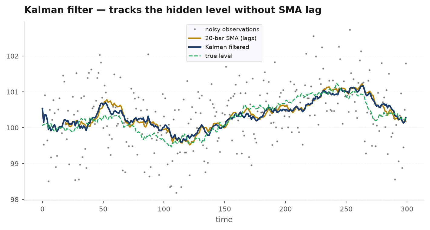
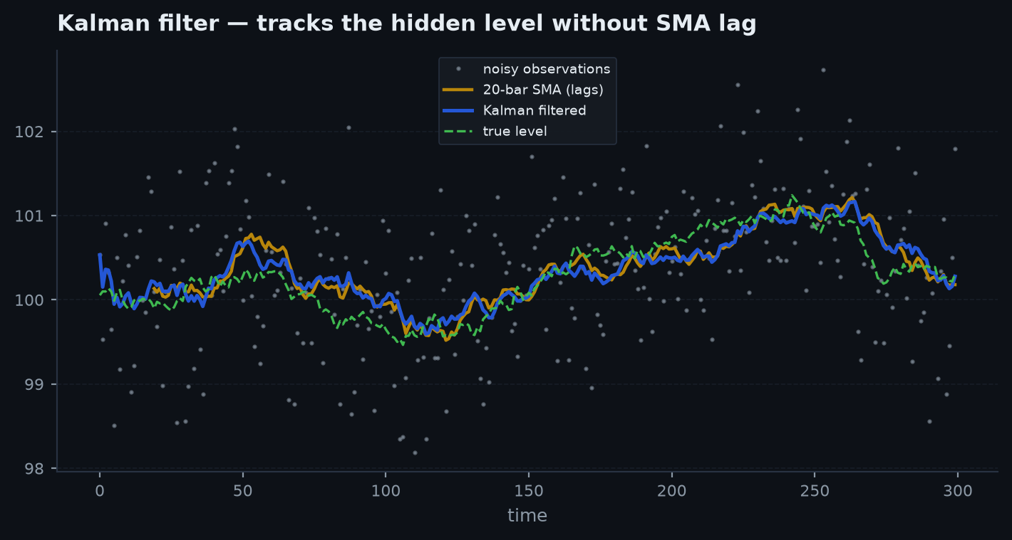
A noisy price series with the Kalman filtered level running through it, tracking turns faster than a moving average of comparable smoothness and shown with a shrinking uncertainty band — Local-level Kalman filter on a noisy series. The filtered mean (smooth line) tracks the hidden level through the noise, adapting at every bar: each estimate is the previous one plus gain times surprise. Unlike a moving average it has no window edge, no fixed lag, and it reports its own variance.

kalman_level.py

import edgekit as ek

# Local-level Kalman filter: hidden random-walk level + observation noise.
# process_var (Q) = how fast the true level drifts; obs_var (R) = how noisy prices are.
# Their ratio sets the effective smoothing — small Q/R = smooth, large = responsive.
level = ek.timeseries.kalman_filter(bars["close"], process_var=1e-5, obs_var=1e-3)
level.tail()          # filtered estimate of the underlying level, one value per bar

Dynamic regression: a beta that breathes#

Now make the hidden state a regression coefficient. Suppose $y_{t}$ (a stock’s return, or one leg of a pair) is driven by $x_{t}$ (the market, or the other leg) through a beta that drifts:

β_{t} = β_{t - 1} + w_{t}, y_{t} = β_{t} x_{t} + v_{t} .

This is still a linear-Gaussian state-space model — the observation matrix is just $H_{t} = x_{t}$ , changing each bar — so the same predict/update cycle applies, with gain $K_{t} = P_{t ∣ t - 1} x_{t} / (x_{t}^{2} P_{t ∣ t - 1} + R)$ and update $β^_{t} = β^_{t ∣ t - 1} + K_{t} (y_{t} - β^_{t ∣ t - 1} x_{t})$ . The result is a time-varying beta estimated causally — at each bar it uses only past data, so it can feed a live strategy without lookahead.

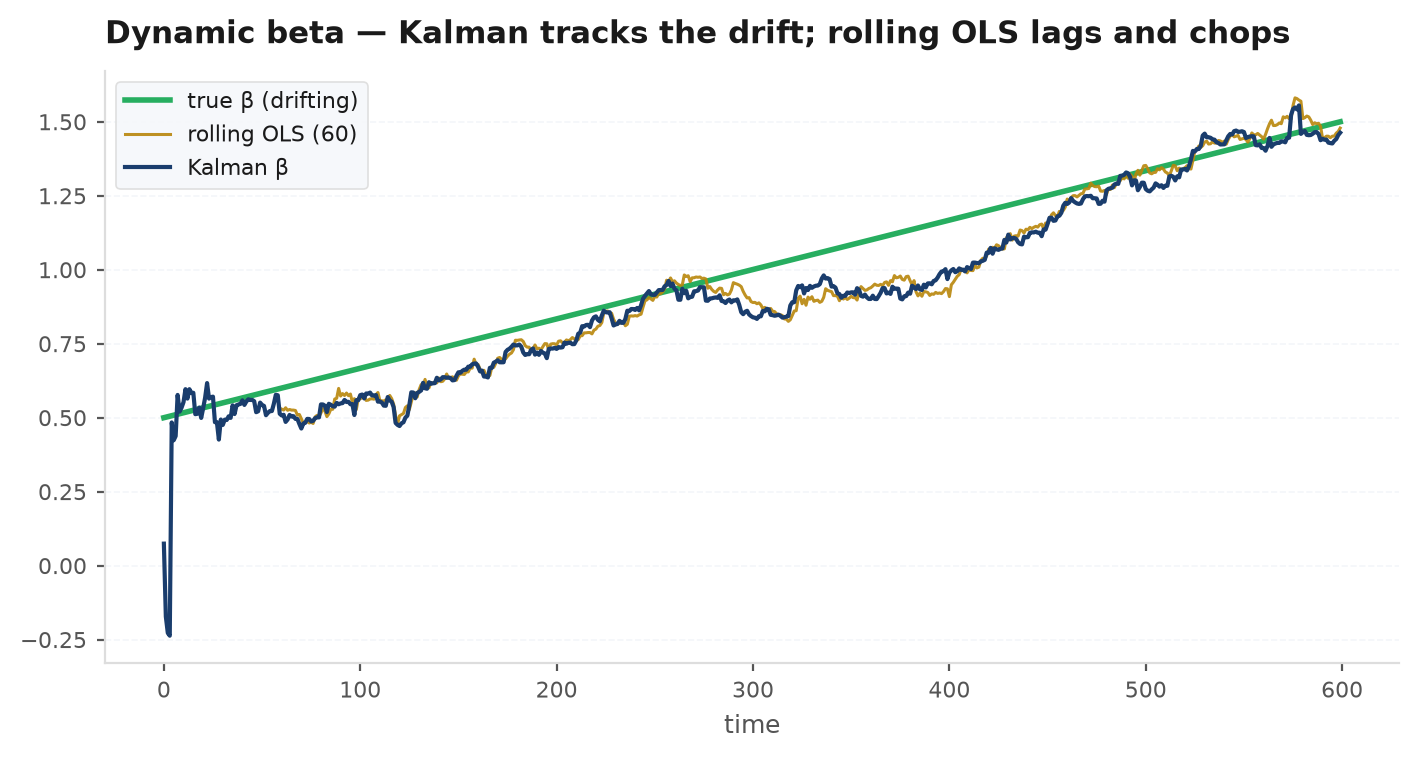
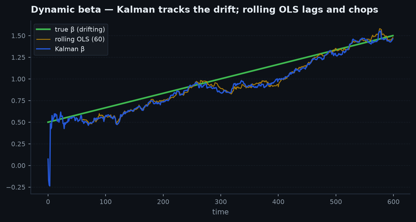
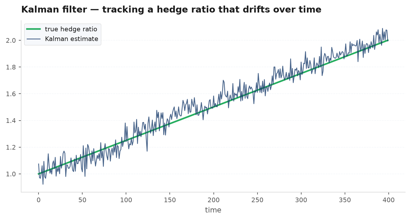
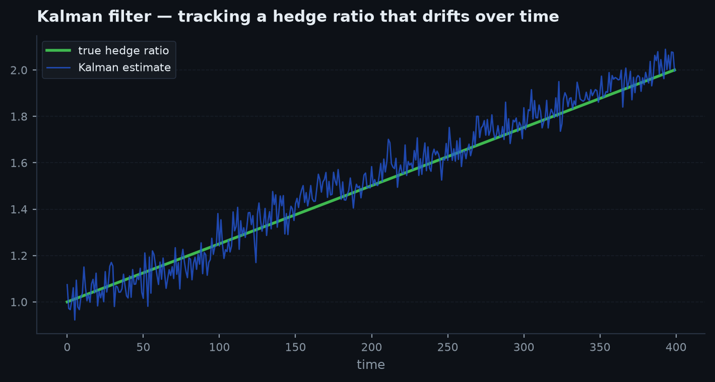
A time-varying regression beta estimated by the Kalman filter, evolving smoothly through a level shift, with a rolling OLS estimate lagging and jumping as the window passes the break — Kalman dynamic beta vs rolling OLS through a structural break. The filter (smooth line) starts adapting the moment the relationship shifts, weighting evidence by recency. Rolling OLS (stepped line) barely moves until the break enters its window, then lurches as old data falls off the cliff edge — a change driven by the calendar, not by new information.

✦Why kalman_hedge beats rolling OLS — no window cliff

The standard alternative is rolling OLS: re-fit the regression on the last $n$ bars. Its flaw is structural. Every observation inside the window has equal weight, and the moment an observation turns $n + 1$ bars old its weight drops from $1/ n$ to zero — the window cliff. A single outlier therefore moves your beta twice: once entering the window, once leaving it, the second time for no economic reason at all. The Kalman filter has no window: influence decays smoothly and geometrically, set by the gain, so the estimate responds to new information and only to new information. For pairs tradingthis matters directly — a hedge ratio that lurches on stale data mis-sizes the spread and manufactures fake z-scores — which is why edgekit’s pairs machinery hedges with kalman_hedge rather than a rolling regression.

Two cointegrated price series and the spread constructed with a Kalman-filtered hedge ratio, remaining stationary while the static-hedge spread drifts — A Kalman-filtered hedge ratio holds a pair’s spread stationary as the relationship drifts. With a static (or cliff-prone rolling) hedge, slow drift in the true ratio leaks trend into the spread and corrupts every z-score built on it.

dynamic_beta.py

import edgekit as ek

y = stock.pct_change().dropna()      # dependent leg
x = market.pct_change().dropna()     # driver

# Time-varying regression coefficient, filtered causally bar by bar.
beta = ek.timeseries.dynamic_beta(y, x, process_var=1e-5, obs_var=1e-3)

# process_var is the knob: raise it and beta adapts faster (trust data);
# lower it and beta stiffens toward a constant OLS-like estimate (trust model).
beta.plot()

Assumptions vs reality#

The Kalman filter assumes	Reality	Consequence
Linear dynamics (A, H)	Relationships bend; betas saturate	Filter tracks the best local linear fit; fine for hedges, wrong for options
Gaussian noise	Fat tails and jumps in returns	A jump reads as huge innovation — the state estimate overreacts
Known Q and R	You must choose or estimate them	Q/R mis-set = over-smoothing or noise-chasing; validate out of sample
Constant noise variances	Volatility clusters (GARCH)	Gain is too high in calm regimes, too low in storms

!The filter believes its model — completely

The Kalman filter is optimal given the state-space model, and silent about whether the model is right. Feed it a structural break it has no state for, and it will dutifully average through the new regime at the old gain. In practice: monitor the innovations. Under the model they should be white noise with the predicted variance; autocorrelated or persistently one-sided innovations are the filter telling you its world-view broke. That check is the state-space cousin of the live-vs-backtest reconciliation in Backtest to live.

Beyond Gaussian: particle filters#

Everything above leans on the Gaussian conjugacy that makes the posterior closed-form. When the model is nonlinear or the noise non-Gaussian — a state that jumps between regimes, stochastic volatility, tail-heavy observation noise — the posterior stops being Gaussian and the Kalman recursion stops being exact. Particle filterskeep the predict/update logic but represent the posterior as a cloud of weighted samples (“particles”): predict by simulating each particle forward through the (arbitrary) state equation, update by re-weighting each particle by its likelihood, and resample when the weights degenerate. The price is Monte-Carlo error and real computational cost; the prize is Bayesian filtering for any state-space model you can simulate. If your innovations diagnostics keep failing Gaussianity, this is the road — via Monte-Carlo methods — but exhaust the linear-Gaussian toolbox first: it is exact, instant, and usually close enough.

Next: the algorithms that make continuous models computable — root-finding, trees, and variance-reduced Monte Carlo — in Numerical methods.