Inequalities & tail bounds

You rarely know the distribution of anything real. What you know is a mean, maybe a variance, maybe that the variable is bounded — and you still have to answer “how likely is disaster?” Probability inequalities are the machinery for saying something rigorous from almost nothing: Markov from a mean, Chebyshev from a variance, Hoeffding from boundedness, Jensen from curvature. This chapter proves each one, shows exactly when each is tight, and works the single most instructive comparison in the subject — one tail probability bounded four different ways.

✦Intuition — a hierarchy of ignorance

Each inequality is a trade: the less you assume, the weaker (but more bulletproof) your conclusion. Know only the mean? Markov gives you a bound that decays like $1/ a$ — feeble, but unconditionally true. Add a variance and Chebyshev buys $1/ a^{2}$ . Add boundedness and Hoeffding buys exponentialdecay — the difference between “a 10-sigma event has probability at most 1%” and “at most $1 0^{- 22}$ ”. Good prep questions walk this ladder deliberately: they hand you minimal information and test whether you reach for the matching rung, and whether you know that each bound is achieved by some worst-case distribution — that nothing stronger is available for free.

Markov — from a mean alone#

Theorem (Markov). If $X \geq 0$ and $a > 0$ , then

P (X \geq a) \leq \frac{E [ X ]}{a} .

✦Proof — one line of truncation

Since $X \geq 0$ , we may discard the part of $X$ below $a$ and floor the rest: $X \geq a 1 {X \geq a}$ pointwise (check both cases: if $X \geq a$ the right side is $a$ ; otherwise it is 0). Take expectations of both sides and use $E [1 {X \geq a}] = P (X \geq a)$ :

E [X] \geq a P (X \geq a) ⟹ P (X \geq a) \leq \frac{E [ X ]}{a} . ■

Sharpness: the bound is achieved by the two-point distribution $P (X = a) = μ / a$ , $P (X = 0) = 1 - μ / a$ — all mass either at zero or exactly at the threshold. No assumption-free improvement exists.

Worked example.A strategy’s daily loss (a non-negative variable on losing days) averages $10k. Markov: the probability of a $100k-plus loss day is at most 10%. Crude — but it required nothingexcept non-negativity and the mean, and it is already enough to falsify a vendor claiming “$100k losses one day in a thousand” while reporting a $10k average loss only if you also trust a variance. Non-negativity is essential: a mean-zero P&L can breach any level with high probability.

Chebyshev — from a variance#

Theorem (Chebyshev). For any $X$ with mean $μ$ and variance $σ^{2}$ , and any $k > 0$ ,

P (∣ X - μ ∣ \geq k σ) \leq \frac{1}{k ^{2}} .

✦Proof — Markov applied to the squared deviation

The variable $(X - μ)^{2}$ is non-negative with mean $σ^{2}$ , so Markov applies to it at level $k^{2} σ^{2}$ :

P (∣ X - μ ∣ \geq k σ) = P ((X - μ)^{2} \geq k^{2} σ^{2}) \leq \frac{E [( X - μ ) ^{2} ]}{k ^{2} σ ^{2}} = \frac{1}{k ^{2}} . ■

The trick generalises: apply Markov to any increasing transform of $∣ X - μ ∣$ . Higher moments give $1/ k^{4}$ and beyond; the exponential transform gives Chernoff below. Sharpness: Chebyshev is achieved by the three-point law $P (X = μ \pm k σ) = \frac{1}{2 k ^{2}}$ , $P (X = μ) = 1 - \frac{1}{k ^{2}}$ — check: the variance is exactly $σ^{2}$ and the tail exactly $1/ k^{2}$ . So the bound is unimprovable in general, yet wildly loose for thin-tailed laws: at $k = 3$ Chebyshev says 11.1% where the normal answer is 0.27%.

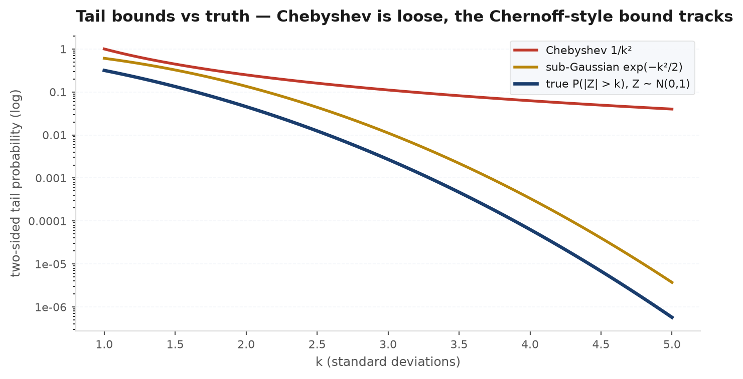
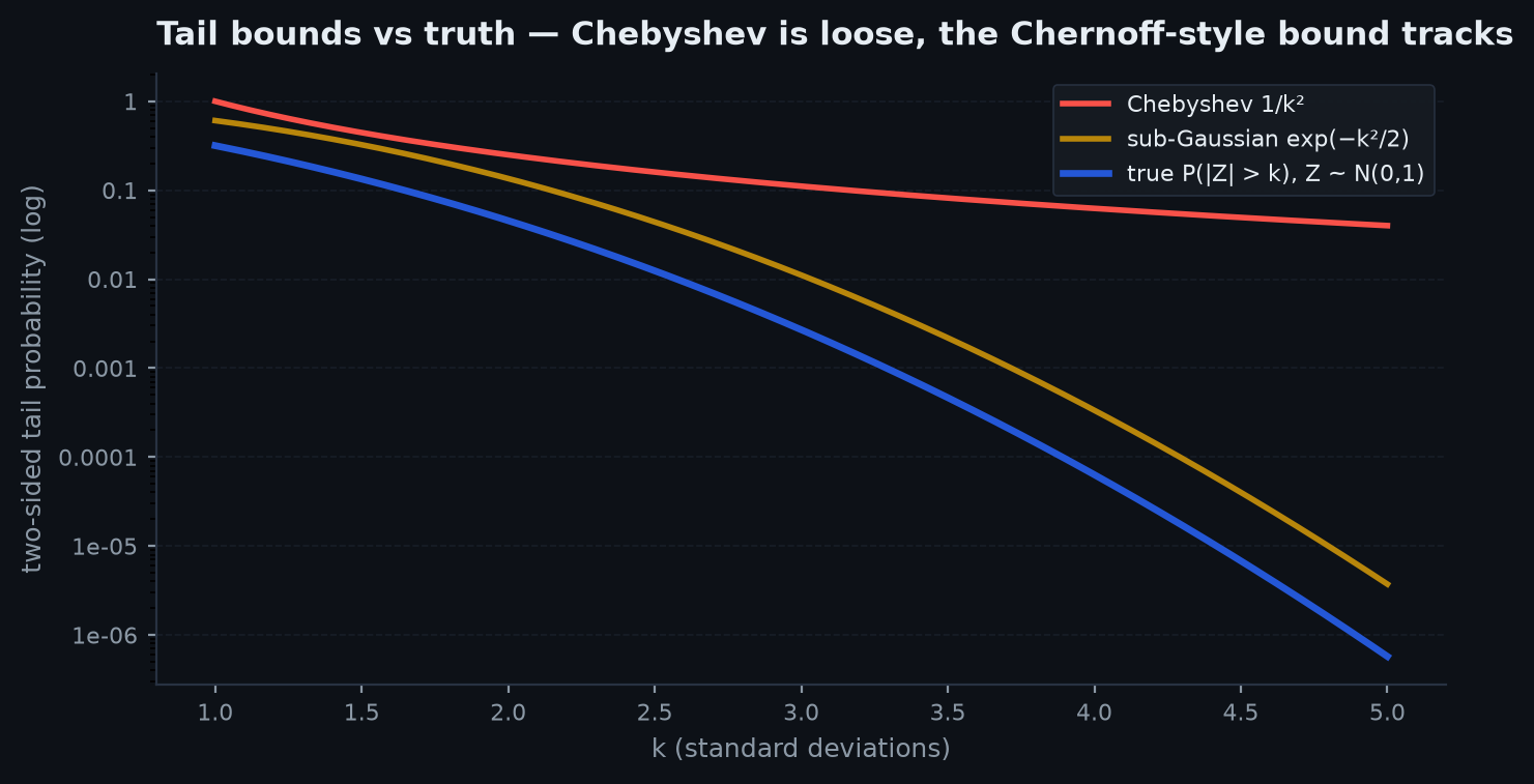
Tail probability versus threshold k for a standard normal, compared against the Chebyshev 1 over k squared bound and a Hoeffding-style exponential bound — Three answers to P(|X - mu| >= k sigma). Chebyshev's 1/k^2 (top) holds for every distribution with that variance; the exponential bound (middle) needs boundedness or subgaussian tails; the exact normal tail (bottom) needs the whole distribution. Information buys decay rate.

One-sided refinement (Cantelli). If only the upper tail matters,

P (X - μ \geq k σ) \leq \frac{1}{1 + k ^{2}},

strictly better than $1/ k^{2}$ for the one-sided question (at $k = 1$ : 50% vs Chebyshev’s vacuous 100%). Sketch: for any $t > 0$ , $X - μ \geq k σ$ implies $(X - μ + t)^{2} \geq (k σ + t)^{2}$ , so Markov gives $P \leq (σ^{2} + t^{2}) / (k σ + t)^{2}$ ; minimise over $t$ (the optimum is $t = σ / k$ ) to get $1/ (1 + k^{2})$ . The free parameter $t$ is a preview of the Chernoff method: introduce a knob, apply Markov, optimise the knob.

Jensen — from curvature#

Theorem (Jensen). If $φ$ is convex, then $φ (E [X]) \leq E [φ (X)]$ ; if concave, the inequality flips. Strict convexity makes it strict unless $X$ is degenerate.

✦Proof — the supporting line (full proof, discrete or not)

Convexity means the graph of $φ$ sits above every tangent (supporting) line. Take the supporting line at the point $μ = E [X]$ : there exists a slope $c$ with

φ (x) \geq φ (μ) + c (x - μ) for all x .

Substitute $x = X$ and take expectations: the linear term dies because $E [X - μ] = 0$ , leaving $E [φ (X)] \geq φ (μ)$ . $■$ (For the discrete two-point case this is literally the definition of convexity, $φ (λ x + (1 - λ) y) \leq λ φ (x) + (1 - λ) φ (y)$ , and induction extends it to any finite mixture — the classical proof; the supporting line does all cases at once.)

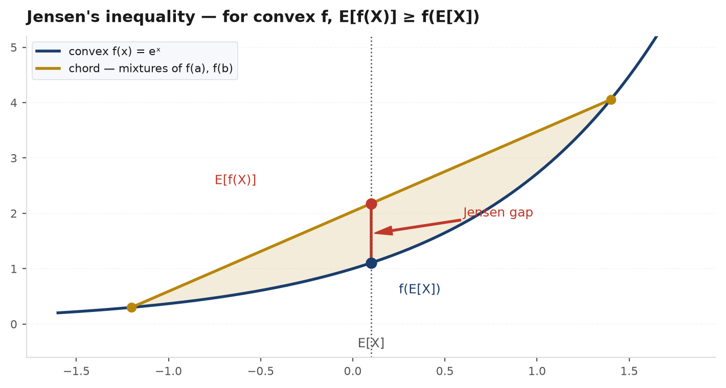
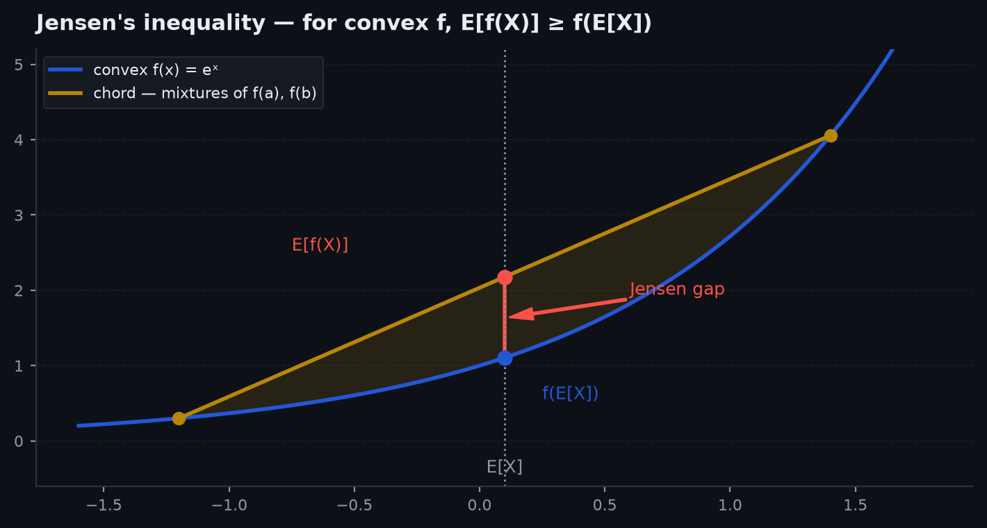
A convex curve with a chord above it connecting two points, showing that the average of the function values sits above the function of the average — Jensen geometrically: for a convex function the chord lies above the curve, so averaging outputs (chord midpoint) beats applying the function to the averaged input (curve). Every vol-drag, E[1/X], and AM-GM fact is this one picture.

Three applications carry most of the practical weight. Reciprocals: $x \mapsto 1/ x$ is convex on $(0, \infty)$ , so $E [1/ X] \geq 1/ E [X]$ — the expected reciprocal of a random discount factor, price relative, or waiting time always exceeds the naive plug-in. Vol drag: $ln$ is concave, so $E [ln (1 + R)] \leq ln (1 + E [R])$ : compound (log) growth is always dragged below the arithmetic mean, the inequality behind the $- σ^{2} /2$ of Itô’s lemma and the lognormal mean/median wedge of the distribution zoo. AM–GM: put a uniform distribution on ${ln a_{1}, \dots, ln a_{n}}$ and exponentiate Jensen for the concave $ln$ :

\frac{1}{n} i \sum ln a_{i} \leq ln (\frac{1}{n} i \sum a_{i}) ⟹ (i \prod a_{i})^{1/ n} \leq \frac{1}{n} i \sum a_{i} .

Cauchy–Schwarz — from second moments#

Theorem. $E [U V]^{2} \leq E [U^{2}] E [V^{2}]$ . Proof: $E [(U - t V)^{2}] \geq 0$ is a quadratic in $t$ with at most one root, so its discriminant is non-positive — which is exactly the claim (equality iff $U$ is a.s. proportional to $V$ ). $■$ Applied to centred variables it bounds covariance by the product of standard deviations, i.e. $∣ ρ ∣ \leq 1$ — the fact used throughout Joint distributions & correlation. A desk-level corollary: the covariance of a signal with returns can never exceed $σ_{signal} σ_{returns}$ , which caps the Sharpe any linear rule built on that signal can achieve — the information-coefficient bound of the math of edge.

Chernoff and Hoeffding — exponential decay#

The Chernoff method is Markov with a tunable exponential lens. For any $t > 0$ , the map $x \mapsto e^{t x}$ is increasing, so

P (X \geq a) = P (e^{tX} \geq e^{t a}) \leq e^{- t a} E [e^{tX}] = e^{- t a} M_{X} (t),

and since this holds for every $t$ , optimise: $P (X \geq a) \leq min_{t > 0} e^{- t a} M_{X} (t)$ . The recipe: (1) exponentiate, (2) Markov, (3) factorise the MGF across independent summands — this is the step where independence pays, because $M_{\sum X_{i}} (t) = \prod_{i} M_{X_{i}} (t)$ turns a sum into a product — then (4) minimise over $t$ . For bounded summands, bounding each MGF by $e^{t^{2} (b_{i} - a_{i})^{2} /8}$ (Hoeffding’s lemma — the honest technical step, proved by a Taylor argument on the log-MGF) yields the celebrated:

Theorem (Hoeffding). If $X_{1}, \dots, X_{n}$ are independent with $X_{i} \in [a_{i}, b_{i}]$ , then for the sample mean $X ˉ$ and any $ε > 0$ ,

P (X ˉ - E [X ˉ] \geq ε) \leq exp (- \frac{2 n ^{2} ε ^{2}}{\sum _{i = 1}^{n} ( b _{i} - a _{i} ) ^{2}}) = [0, 1] e^{- 2 n ε^{2}} .

Interpretation: the sample mean of bounded variables concentrates around the truth at an exponential rate — no normality assumed, no asymptotics, valid at every finite $n$ . Doubling the sample squares the tail probability. This is the rigorous, non-asymptotic cousin of the CLT: the CLT tells you the shapeof the fluctuation, Hoeffding gives a certificate against being fooled by it. Berry–Esseen (next chapter) quantifies how fast the CLT shape itself becomes trustworthy — error $\leq 0.4748 ρ_{3} / (σ^{3} n)$ in the CDF, so with skewed trade P&L the Gaussian approximation converges at only $1/ n$ .

Worked example — how long a backtest? Trades are wins or losses (bounded in $[0, 1]$ after coding a win as 1). You want the observed win rate within $ε = 3%$ of truth with 95% confidence. Two-sided Hoeffding: $2 e^{- 2 n (0.03)^{2}} \leq 0.05$ gives $n \geq ln (40) / (2 \times 0.0009) \approx 2, 050$ trades. A claimed edge of 53% vs 50% needs thousands of trades before the data can certify it — arithmetic that should precede every backtest read-out, and the reason the gauntlet demands sample-size honesty before it looks at a Sharpe ratio.

The union bound — and its multiple-testing sting#

Theorem (Boole). For any events (no independence needed), $P (⋃_{i = 1}^{n} A_{i}) \leq \sum_{i = 1}^{n} P (A_{i})$ . Proof: induction from two events, where $P (A \cup B) = P (A) + P (B) - P (A \cap B) \leq P (A) + P (B)$ by the inclusion–exclusion identity of Counting & combinatorics; alternatively note the indicator of the union is pointwise at most the sum of indicators and take expectations. $■$

The sting: test 20 useless strategies at the 5% level and the union bound caps the chance that some strategy passes at $20 \times 0.05 = 1$ — vacuous, and under independence the true probability is $1 - 0.9 5^{20} \approx 64%$ . Flip it into a control: to keep the family-wise error below $α$ across $n$ tests, test each at $α / n$ — the Bonferroni correction, proved by exactly this bound and developed with its refinements in Multiple testing & paradoxes. Combined with Hoeffding it also prices the maximum of many strategies’ luck — Problem 5 below.

Bound	Requires	Tail decay	Tight when
Markov	$X \geq 0, E [X]$	$1/ a$	mass at 0 and at the threshold
Chebyshev	$μ, σ^{2}$	$1/ k^{2}$	three-point worst case
Cantelli	$μ, σ^{2}$	$1/ (1 + k^{2})$	one-sided questions
Jensen	convexity of φ	— (moment inequality)	φ linear, or X degenerate
Hoeffding / Chernoff	independence + boundedness (or MGF)	$e^{- 2 n ε^{2}}$	near-Gaussian bounded sums
Union bound	nothing	additive	rare, nearly disjoint events

A seeded simulation runs the whole ladder on one target — a fair coin showing at least 60% heads in 100 flips — against the exact answer computed in Problem 2:

bounds_ladder.py

import numpy as np
from math import comb, exp, sqrt

rng = np.random.default_rng(11)

# Target: P(at least 60 heads in 100 fair flips)
n, p, k = 100, 0.5, 60
exact = sum(comb(n, j) for j in range(k, n + 1)) / 2**n
cheb = (p * (1 - p) / n) / 0.10**2          # Chebyshev, two-sided /2 not taken
cantelli = 1 / (1 + 0.10**2 * n / (p * (1 - p)))
hoeff = exp(-2 * n * 0.10**2)
# CLT with continuity correction: P(Z > (59.5 - 50)/5)
from math import erfc
clt = 0.5 * erfc((59.5 - 50) / 5 / sqrt(2))

sim = (rng.binomial(n, p, 2_000_000) >= k).mean()
print(f"exact    {exact:.5f}")   # 0.02844
print(f"sim      {sim:.5f}")     # ~0.0284
print(f"clt      {clt:.5f}")     # 0.02871  (continuity-corrected)
print(f"hoeffding{hoeff: .5f}")  # 0.13534  (valid bound, ~5x loose)
print(f"cantelli {cantelli:.5f}")# 0.71429  (loose)
print(f"chebyshev{cheb: .5f}")   # 2.50000  (vacuous here)

→Quant lens — bounds are risk statements you can sign

A model-based tail estimate (“VaR says 1%”) is only as good as the fitted distribution — and fitted distributions lieprecisely in the tails. Inequality-based statements are different in kind: “with only the variance assumed, the loss exceeds

3 σ

with probability at most 11%” survives any distributional surprise, fat tails included. Desks use the ladder in both directions: Chebyshev-style bounds for worst-case risk language when tails are untrusted, and Hoeffding-style concentration for certification — how many trades before a win rate, hit ratio, or A/B execution improvement is believable. The habit to build: before quoting any backtest statistic, ask which rung of the ladder your sample size actually supports.

Practice problems#

→Problem 1 — Bound P(X ≥ 2μ)

A non-negative random variable has mean $μ$ . (a) Bound $P (X \geq 2 μ)$ . (b) Show the bound cannot be improved. (c) If you also learn $Var (X) = μ^{2} /4$ , improve it.

Solution. (a) Markov: $P (X \geq 2 μ) \leq μ /2 μ = 1/2$ . (b) Take $P (X = 2 μ) = 1/2, P (X = 0) = 1/2$ : the mean is $μ$ and the tail is exactly $1/2$ — Markov is tight, so without more information $1/2$ is the honest answer. (c) With a variance, use one-sided Cantelli with $k σ = μ$ , i.e. $k = μ / σ = 2$ :

P (X - μ \geq μ) \leq \frac{1}{1 + k ^{2}} = \frac{1}{5} = 0.2,

a 2.5× improvement from one extra number (plain Chebyshev would give $1/4$ , and wastes half its budget on the impossible lower tail). The escalation pattern — quote Markov, prove tightness, then upgrade when handed the variance — is exactly the ladder-climbing these problems are built to exercise.

→Problem 2 — 60% heads in 100 flips: Hoeffding vs CLT vs exact

A fair coin is flipped 100 times. Estimate $P (at least 60 heads)$ three ways and reconcile.

Solution. Hoeffding (a bound): $P (X ˉ - 0.5 \geq 0.1) \leq e^{- 2 \cdot 100 \cdot 0.01} = e^{- 2} \approx 0.135$ . CLT (an approximation): $σ_{X ˉ} = 0.05$ , so 60% is 2 standard errors out; with continuity correction, $P \approx P (Z \geq 1.9) \approx 0.029$ . Exact: $2^{- 100} \sum_{k = 60}^{100} (k 100) \approx 0.0284$ . Reconciliation: the exact answer is the truth; the CLT is a superb approximation here (symmetric, thin-tailed summands, decent $n$ ) but carries no guarantee; Hoeffding is 5× loose but is a certificate valid for every bounded distribution and every $n$ . Knowing which of the three to reach for — and saying so unprompted — is the real mark of understanding.

→Problem 3 — Jensen traps: E[S²] vs E[S]², and friends

True or false, with proof: (a) $E [S^{2}] \geq E [S]^{2}$ ; (b) for positive $S$ , $E [1/ S] = 1/ E [S]$ ; (c) the expected Sharpe of a strategy equals the Sharpe of its expected returns; (d) $E [S] \geq E [S]$ .

Solution. (a) True — $x^{2}$ is convex; the gap $E [S^{2}] - E [S]^{2}$ is precisely the variance, so equality holds iff $S$ is constant. (b) False — $1/ x$ is convex, so $E [1/ S] \geq 1/ E [S]$ , strictly unless degenerate. Concretely, $S \in {1, 3}$ equiprobable: $E [1/ S] = 2/3 > 1/2$ . (c) False in general — the Sharpe is a nonlinear (concave-in-places) function of estimated moments; noisy estimates bias it, one reason reported backtest Sharpes flatter. (d) False as stated — $x$ is concave, so the inequality runs the other way: $E [S] \leq E [S]$ (this is also why $s = s^{2}$ underestimates $σ$ even when $s^{2}$ is unbiased — see Estimators & sampling theory). The meta-rule: identify convex vs concave, and Jensen dictates the direction; the size of the gap always scales with variance.

→Problem 4 — How big is the max of n Gaussians?

$Z_{1}, \dots, Z_{n}$ are standard normal (not necessarily independent). Show $E [max_{i} Z_{i}] \leq 2 ln n$ , and argue the rate is right.

Solution. The slick proof is Jensen + union-bound logic through the MGF. For any $t > 0$ :

e^{t E [m a x Z_{i}]} \leq E [e^{t m a x Z_{i}}] = E [i max e^{t Z_{i}}] \leq i = 1 \sum n E [e^{t Z_{i}}] = n e^{t^{2} /2} .

Take logs: $E [max Z_{i}] \leq ln n / t + t /2$ ; minimise at $t = 2 ln n$ to get $E [max Z_{i}] \leq 2 ln n$ — with no independence used anywhere. For iid Gaussians the bound is asymptotically exact (the tail $P (Z > z) \approx φ (z) / z$ puts the top order statistic near $2 ln n$ ), so the rate is correct: the best of $n$ lucky draws grows only like $ln n$ — slowly, but never zero. Numbers worth carrying: $n = 20$ gives about 2.4; $n = 1000$ about 3.7.

→Problem 5 — The best of N random strategies

A fund tries $N = 100$ strategies with no true edge; each backtest Sharpe is approximately $N (0, 1/ T^{2} \cdot T) = N (0, 1)$ after scaling by $T$ years. How good will the best backtest look, and how many strategies until a “2.5-Sharpe-t-stat” discovery is expected by chance?

Solution. By Problem 4, the expected best t-stat is about $2 ln 100 \approx 3.03$ — a “three-sigma discovery” manufactured from pure noise. For the second part, the union bound (or independence) says a level- $z$ exceedance is expected once $N \cdot P (Z > z) \approx 1$ : with $P (Z > 2.5) \approx 0.0062$ , about $N \approx 160$ strategies suffice — an afternoon of parameter search. This $2 ln N$ arithmetic is the entire mathematical core of data snooping: the more you search, the better your best must look, edge or not. Corrections (Bonferroni, deflated Sharpe) live in Multiple testing & paradoxes and Overfitting detection.

Next: concentration bounds say averages settle; the limit theorems say how — the law of large numbers gives the destination and the central limit theorem the shape of the journey, including the exact arithmetic of how many trades an edge needs. LLN & the central limit theorem.