Generating functions

A generating function packs an entire distribution into one function: $G (s) = E [s^{X}]$ hangs every probability $P (X = k)$ on the coefficient of $s^{k}$ , like laundry on a clothesline, and hard operations on distributions become easy operations on functions: convolution becomes multiplication, random sums become composition, recursions become algebra. This chapter builds the PGF toolkit, factorises dice, finds branching-process extinction as a fixed point, situates MGFs and characteristic functions, and closes by solving a Fibonacci-flavoured coin-flip recursion in three lines.

✦Intuition — one function, whole distribution; algebra instead of convolution

A discrete distribution is an infinite list of numbers, and lists are clumsy: adding two independent random variables forces you to convolve them — $P (X + Y = k) = \sum_{j} P (X = j) P (Y = k - j)$ , a fresh sum for every $k$ . The generating function trades the list for the single object $G (s) = \sum_{k} p_{k} s^{k}$ , and the dummy variable $s$ does the bookkeeping: multiplying power series automatically convolves coefficients, because $s^{j} \cdot s^{k - j} = s^{k}$ . Everything here is that idea worn four ways: encode the distribution so that summing, mixing, compounding, or recursing becomes algebra on $G$ .

The clothesline: definition and first properties#

For a random variable $X$ taking values in ${0, 1, 2, \dots}$ , the probability generating function is

G_{X} (s) = E [s^{X}] = k \geq 0 \sum P (X = k) s^{k}, ∣ s ∣ \leq 1,

convergent there since the coefficients are probabilities. Three facts fall out immediately:

Normalisation: $G (1) = \sum_{k} p_{k} = 1$ — every PGF passes through $(1, 1)$ .
Recovery: $P (X = k) = G^{(k)} (0) / k!$ — Taylor’s theorem reads probabilities back off the clothesline; in particular $P (X = 0) = G (0)$ , which the branching-process section leans on hard.
Uniqueness: a power series determines its coefficients, so $G_{X} = G_{Y}$ forces $X = d Y$ — to prove two distributions equal, match their PGFs.

Moments come from derivatives at $s = 1$ — the second derivative delivers the factorial moment, since differentiating $s^{k}$ twice produces $k (k - 1)$ , and the variance formula repairs the difference:

E [X] = G^{'} (1), E [X (X - 1)] = G^{''} (1), Var (X) = G^{''} (1) + G^{'} (1) - G^{'} (1)^{2} .

✦Worked example — the four standard PGFs, derived

Bernoulli( $p$ ): $G (s) = q + p s$ with $q = 1 - p$ — a one-rung clothesline. Binomial( $n, p$ ): $\sum_{k} (k n) p^{k} q^{n - k} s^{k} = (q + p s)^{n}$ by the binomial theorem — or wait one section and get it for free from independence. Geometric( $p$ ) on ${1, 2, \dots}$ (trials to first success): $G (s) = \sum_{n \geq 1} q^{n - 1} p s^{n} = p s \sum_{n \geq 1} (q s)^{n - 1} = \frac{p s}{1 - q s}$ ; check $G^{'} (1) = 1/ p$ , the familiar mean from common distributions. Poisson( $λ$ ): $G (s) = \sum_{k \geq 0} e^{- λ} \frac{λ ^{k}}{k !} s^{k} = e^{- λ} e^{λ s} = e^{λ (s - 1)}$ ; then $G^{'} (1) = λ$ and $G^{''} (1) = λ^{2}$ give $Var = λ^{2} + λ - λ^{2} = λ$ — index gymnastics replaced by a one-line differentiation.

Independence means multiply#

The theorem that earns the whole machine: for independent $X$ and $Y$ ,

G_{X + Y} (s) = E [s^{X + Y}] = E [s^{X}] E [s^{Y}] = G_{X} (s) G_{Y} (s),

because independence factorises the expectation of $s^{X} \cdot s^{Y}$ . Compare the convolution slog of transformations of random variables: there, a sum cost a fresh summation for every value; here, one multiplication for all values at once. Two showpieces:

Binomial = product of Bernoullis. A Binomial( $n, p$ ) count is a sum of $n$ independent Bernoullis, so its PGF is $(q + p s)^{n}$ — no binomial theorem needed.
Sum of independent Poissons is Poisson. $e^{λ (s - 1)} \cdot e^{μ (s - 1)} = e^{(λ + μ) (s - 1)}$ , the Poisson( $λ + μ$ ) PGF — uniqueness finishes the proof. The direct convolution route needs a Vandermonde-style binomial sum; the PGF route adds two exponents. This additivity is why two independent order-flow streams merge into one Poisson stream at the summed rate.

!Multiplication needs independence

The implication runs from independence to factorisation, not back — and the PGF of a sum records the sum’s distributiononly, forgetting joint structure. Two portfolios can have identical P&L distributions with wildly different co-movement; keep joint distributions in the toolkit.

The dice factorisation showpiece#

Generating functions turn dice questions into polynomial questions — and polynomial factorisation is a solved subject. Two classics, worked fully.

✦Proof — you cannot weight two dice to make all sums equally likely

Can you load two six-sided dice (any face probabilities) so that the sum is uniform on ${2, \dots, 12}$ , each sum with probability $1/11$ ? Writing the dice PGFs $A (s) = \sum_{i} a_{i} s^{i}$ , $B (s) = \sum_{i} b_{i} s^{i}$ , uniformity demands

A (s) B (s) = \frac{1}{11} (s^{2} + s^{3} + \dots + s^{12}) = \frac{s ^{2}}{11} \frac{s ^{11} - 1}{s - 1} .

Reaching sums 2 and 12 forces $a_{1}, b_{1}, a_{6}, b_{6} > 0$ , so $A (s) = s A_{1} (s)$ , $B (s) = s B_{1} (s)$ with $A_{1}, B_{1}$ real polynomials of degree exactly 5, and $A_{1} (s) B_{1} (s) = \frac{1}{11} (1 + s + \dots + s^{10})$ . The killer observation: $A_{1}$ has odd degree, and every real polynomial of odd degree has a real root. But the roots of $1 + s + \dots + s^{10} = \frac{s ^{11} - 1}{s - 1}$ are the eleventh roots of unity other than 1 — none of them real. Contradiction. $■$ A fact about all possible dice, proved by looking at eleven complex numbers on a circle.

✦Worked example — Sicherman dice: refactorising the standard sum

The standard die has face polynomial $d (s) = s + s^{2} + \dots + s^{6}$ (PGF times 6), which factorises over the integers as

d (s) = s (1 + s) (1 + s + s^{2}) (1 - s + s^{2}) .

Two standard dice give the sum polynomial $d (s)^{2}$ — each factor twice. Any pair with the same sum distribution must split these eight factors into two polynomials with non-negative coefficients, value 6 at $s = 1$ (six faces), and no constant term (positive faces). At $s = 1$ the factors evaluate to $1, 2, 3, 1$ , so each die takes one $s$ , one $(1 + s)$ , one $(1 + s + s^{2})$ ; the only freedom is where the two $(1 - s + s^{2})$ factors go. One each recovers the standard dice; both on one die gives

A (s) = s (1 + s) (1 + s + s^{2}) = s + 2 s^{2} + 2 s^{3} + s^{4}, B (s) = \frac{d ( s ) ^{2}}{A ( s )} = s + s^{3} + s^{4} + s^{5} + s^{6} + s^{8} .

Faces ${1, 2, 2, 3, 3, 4}$ and ${1, 3, 4, 5, 6, 8}$ — the Sicherman dice, the unique non-standard pair of positive-integer-faced dice whose sum matches two ordinary dice. Sum-7 check: six of 36 pairs, $6/36 = 1/6 \approx 0.1667$ , exactly the standard count. Distribution problems became factor bookkeeping.

Random sums: composition#

Sum a random number of terms: $S_{N} = X_{1} + \dots + X_{N}$ , the $X_{i}$ i.i.d. with PGF $G_{X}$ , $N$ an independent count with PGF $G_{N}$ — losses over a random number of claims, fills over a random number of child orders:

G_{S_{N}} (s) = G_{N} (G_{X} (s)) .

✦Proof — condition on N and use the tower rule

Condition on $N$ and apply the tower property from conditional expectation:

E [s^{S_{N}}] = E [E [s^{X_{1} + \dots + X_{N}} ∣ N]] = E [(G_{X} (s))^{N}] = G_{N} (G_{X} (s)),

where the middle equality uses independence — given $N = n$ , the inner expectation is $G_{X} (s)^{n}$ — and the last is the definition of $G_{N}$ evaluated at the number $G_{X} (s)$ . $■$ Differentiate at $s = 1$ with the chain rule, using $G_{X} (1) = 1$ : $G_{S_{N}}^{'} (1) = G_{N}^{'} (1) G_{X}^{'} (1)$ — Wald’s identity $E [S_{N}] = E [N] E [X]$ in one stroke. Compare the stopping-time proof in martingales & optional stopping, which allows $N$ to depend on the summands. A second differentiation gives $Var (S_{N}) = E [N] Var (X) + Var (N) E [X]^{2}$ .

Branching processes and extinction#

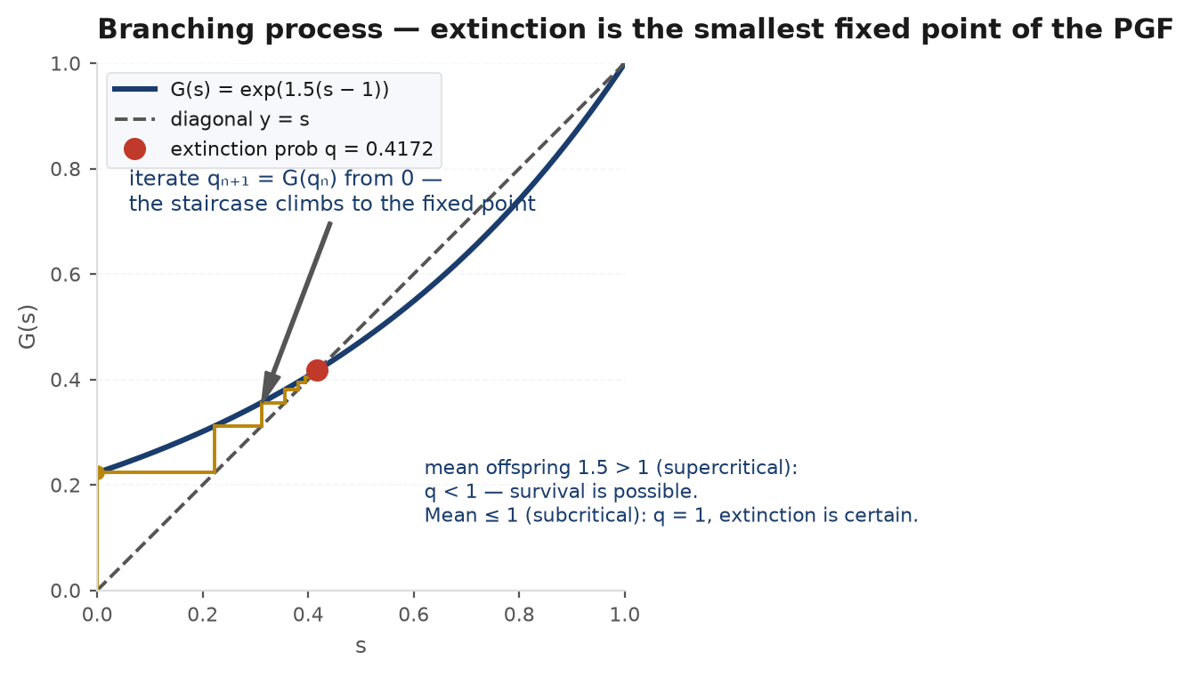
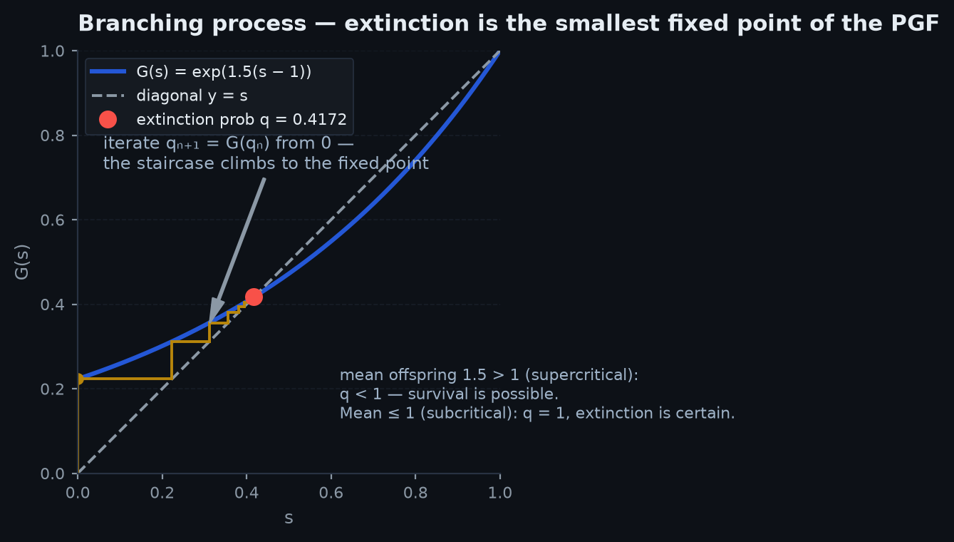
The deepest application of composition. A branching process starts with one individual ( $Z_{0} = 1$ ); each independently produces offspring with PGF $G$ and mean $m = G^{'} (1)$ . Generation sizes obey $Z_{n + 1} = \sum_{i = 1}^{Z_{n}} X_{i}$ — a random sum — so the PGF of $Z_{n}$ is the $n$ -fold composition $G_{n} = G \circ \dots \circ G$ . Does the line die out? Since $P (Z_{n} = 0) = G_{n} (0)$ , extinction by generation $n$ is literally iterating $G$ from 0.

✦Proof sketch — extinction probability is the smallest fixed point of s = G(s)

The events ${Z_{n} = 0}$ increase (an extinct line stays extinct), so $q_{n} = G_{n} (0) ↑ q$ , the extinction probability, by continuity of probability; and since $q_{n + 1} = G (q_{n})$ with $G$ continuous, $q = G (q)$ . It is the smallest fixed point in $[0, 1]$ : for any $r = G (r)$ , induction with the monotonicity of $G$ (non-negative coefficients) gives $q_{n + 1} = G (q_{n}) \leq G (r) = r$ , so $q \leq r$ . $■$

The trichotomy comes from convexity: $G^{''} \geq 0$ , so the curve crosses the diagonal at most twice, always passing through $(1, 1)$ with slope $m$ . If $m \leq 1$ (subcritical or critical) the curve stays above the diagonal on $[0, 1)$ and $q = 1$ : extinction is certain — even at $m = 1$ , where the population is a martingale yet still dies (excluding the degenerate one-child-always case). If $m > 1$ (supercritical), the curve dips below the diagonal near 1 and picks up a second crossing at some $q < 1$ : survival has positive probability $1 - q$ .

For Poisson( $1.5$ ) offspring, $G (s) = e^{1.5 (s - 1)}$ and $m = 1.5 > 1$ : supercritical. The fixed-point equation $q = e^{1.5 (q - 1)}$ has no closed form, but iterating from 0 converges fast: $q_{1} = e^{- 1.5} \approx 0.223$ , $q_{2} \approx 0.312$ , … $\to q \approx 0.417$ . Each iterate is a probability — extinct by generation $n$ — so the staircase below is the population’s life history, one generation per step.

Cobweb diagram iterating s to G(s) for Poisson(1.5) offspring: the convex PGF curve crosses the diagonal at the extinction probability q below one, and the iteration staircase from zero climbs to q — The cobweb of extinction: iterating s ↦ G(s) from s = 0 for Poisson(1.5) offspring. Each iterate G_n(0) equals P(extinct by generation n), so the staircase climbing between curve and diagonal traces the extinction probabilities generation by generation, converging monotonically to the smallest fixed point q ≈ 0.417 — not to the other fixed point at 1, which the supercritical slope G′(1) = 1.5 > 1 makes repelling.

→Quant lens — cascades, contagion, and the life of an edge

Branching arithmetic runs anything that spreads by replication. An order-book message cascade — one aggressive order triggers algos whose reactions trigger more — has offspring mean $m$ = average follow-on messages per message: at $m < 1$ bursts die fast; near 1 cascade sizes grow heavy tails; past 1 you get flash-crash dynamics that need not damp. Default contagion reads the same way, and — a lighter analogy — a trading edge spawning copycats each “generation” dies out with certainty when $m \leq 1$ but crowds permanently with probability $1 - q$ when $m > 1$ . The moral is the trichotomy itself: the qualitative fate of the whole system is decided by a first derivative crossing 1.

branching_extinction.py

import numpy as np

rng = np.random.default_rng(42)
lam = 1.5  # Poisson offspring mean (supercritical: m = 1.5 > 1)

# Fixed point of s = exp(lam*(s-1)): iterate G from 0.
q = 0.0
for _ in range(200):
    q = np.exp(lam * (q - 1.0))

def goes_extinct(max_gen=100, cap=10_000):
    z = 1
    for _ in range(max_gen):
        z = rng.poisson(lam, size=z).sum()
        if z == 0:
            return True
        if z > cap:  # this large essentially never dies
            return False
    return False

freq = np.mean([goes_extinct() for _ in range(20_000)])
print(f"simulated extinction frequency : {freq:.4f}")
print(f"fixed point of s = e^(lam(s-1)) : {q:.4f}")
# Expected: both extinction numbers near 0.4172.

MGFs, Chernoff, and characteristic functions#

The moment generating function $M (t) = E [e^{tX}]$ is the PGF in different clothes — substitute $s = e^{t}$ — but works for continuous and negative-valued variables too. Expanding the exponential, $M (t) = \sum_{n \geq 0} E [X^{n}] t^{n} / n!$ : the clothesline now hangs moments, $E [X^{n}] = M^{(n)} (0)$ , and independence still multiplies: $M_{X + Y} = M_{X} M_{Y}$ .

✦Worked example — the normal MGF, by completing the square

For $X \sim N (μ, σ^{2})$ , write $X = μ + σ Z$ and compute for standard $Z$ :

E [e^{tZ}] = \int \frac{e ^{t z - z^{2} /2}}{2 π} d z = e^{t^{2} /2} \int \frac{e ^{- (z - t)^{2} /2}}{2 π} d z = e^{t^{2} /2},

since $t z - z^{2} /2 = - \frac{1}{2} (z - t)^{2} + \frac{1}{2} t^{2}$ and the shifted Gaussian still integrates to 1. Hence $M_{X} (t) = e^{μ t + σ^{2} t^{2} /2}$ : sums of independent normals are normal (exponents add), and every normal moment is a coefficient — the $t^{4}$ coefficient $1/8 = E [Z^{4}] /4!$ gives $E [Z^{4}] = 3$ .

The MGF is also the Chernoff engine: Markov’s inequality applied to $e^{tX}$ gives $P (X \geq a) \leq e^{- t a} M (t)$ for any $t > 0$ , and optimising over $t$ produces exponentially decaying tail bounds — worked in full in inequalities & tail bounds. One caveat: MGFs can fail to exist — $E [e^{tX}]$ is infinite for every $t > 0$ when $X$ is lognormal (see common distributions): tails heavier than exponential kill the integral. One repair: the characteristic function $φ (t) = E [e^{i tX}]$ always exists ( $∣ e^{i tX} ∣ = 1$ is bounded) and keeps every virtue — uniqueness, multiplication under independence, moments from derivatives. It is how the CLT is actually proved: the sketch in LLN & CLT is a second-order Taylor expansion of $φ$ raised to the $n$ -th power.

Solving recursions: no two heads in a row#

The last hat generating functions wear: solving recursions. How many length- $n$ H/T sequences contain no two consecutive heads? Condition the count $a_{n}$ on the last flip: ending in T leaves any valid string of length $n - 1$ ; ending in H forces a preceding T, leaving length $n - 2$ . So $a_{n} = a_{n - 1} + a_{n - 2}$ with $a_{1} = 2, a_{2} = 3$ (set $a_{0} = 1$ ): Fibonacci in disguise, $a_{n} = F_{n + 2}$ . Multiply by $x^{n}$ , sum over $n \geq 2$ , and solve for $A (x) = \sum_{n} a_{n} x^{n}$ :

A (x) - 1 - 2 x = x (A (x) - 1) + x^{2} A (x) ⟹ A (x) = \frac{1 + x}{1 - x - x ^{2}} .

Partial fractions over the roots of $1 - x - x^{2}$ give $a_{n} \sim c φ^{n}$ with $φ = (1 + 5) /2 \approx 1.618$ — surviving $n$ fair flips without HH decays like $(φ /2)^{n} \approx 0.80 9^{n}$ . Now the pivot to waiting times: if $N$ is the flip on which HH first completes, ${N > n}$ is exactly “no HH in the first $n$ flips,” so $P (N > n) = a_{n} / 2^{n}$ , and the tail-sum formula from random variables & moments evaluates the expectation as the generating function at a point:

E [N] = n \geq 0 \sum P (N > n) = n \geq 0 \sum \frac{a _{n}}{2 ^{n}} = A (\frac{1}{2}) = \frac{1 + \frac{1}{2}}{1 - \frac{1}{2} - \frac{1}{4}} = \frac{3/2}{1/4} = 6.

Six flips on average to see HH — agreeing, by a completely different route, with the overlap formula $2^{2} + 2 = 6$ from the ABRACADABRA argument in martingales & optional stopping. The full distribution comes too: $\sum_{n \geq 0} P (N > n) s^{n} = \frac{1 - G _{N} ( s )}{1 - s}$ inverts to $G_{N} (s) = 1 - (1 - s) A (s /2) = \frac{s ^{2}}{4 - 2 s - s ^{2}}$ — check $G_{N} (1) = 1$ , $P (N = 2) = 1/4$ — the clothesline, fully loaded.

Practice problems#

Five problems to test understanding — each turns into algebra once you write the right generating function.

→Problem 1 — a specific probability for the sum of three dice

Write the PGF of one fair die and of the sum of $k$ dice; compute $P (sum of 3 dice = 10)$ .

Solution. One die: $D (s) = \frac{1}{6} (s + \dots + s^{6}) = \frac{s}{6} \cdot \frac{1 - s ^{6}}{1 - s}$ ; $k$ dice: $D (s)^{k}$ by independence. For $k = 3$ we need the $s^{7}$ coefficient of $(1 - 3 s^{6} + \dots) \sum_{m} (2 m + 2) s^{m}$ , over 216: $m = 7$ gives $(2 9) = 36$ , the $- 3 s^{6}$ term with $m = 1$ gives $- 9$ , so $P = 27/216 = 1/8 = 0.125$ . The machinery replaced enumerating 27 ordered triples — and scales to 10 dice, where enumeration does not.

→Problem 2 — geometrics sum to negative binomial

Show via PGFs that the sum of $r$ independent Geometric( $p$ ) variables is negative binomial, and read off its pmf.

Solution. Multiply PGFs: $G_{S} (s) = (\frac{p s}{1 - q s})^{r}$ . Expand with the generalised binomial series $(1 - q s)^{- r} = \sum_{j \geq 0} (j r + j - 1) (q s)^{j}$ : the coefficient of $s^{n}$ (with $n = r + j$ ) is $(r - 1 n - 1) p^{r} q^{n - r}$ — the negative binomial pmf: the first $n - 1$ trials hold $r - 1$ successes, and trial $n$ is the $r$ -th. The PGF proves in two lines what convolution proves in a page — the combinatorial reading falls out of the algebra.

→Problem 3 — a compound Poisson claim total

Claims arrive as $N \sim Poisson (2)$ ; each claim size is independently Geometric( $\frac{1}{2}$ ) on ${1, 2, \dots}$ . Find the PGF of the total $S$ , then $E [S]$ and $P (S = 0), P (S = 1)$ .

Solution. Composition: $G_{X} (s) = \frac{s}{2 - s}$ , so $G_{S} (s) = G_{N} (G_{X} (s)) = exp (2 (\frac{s}{2 - s} - 1))$ . Wald: $E [S] = 2 \times 2 = 4$ . Atoms: $P (S = 0) = G_{S} (0) = e^{- 2} \approx 0.1353$ — exactly $P (N = 0)$ , since every claim is at least 1; and $P (S = 1) = G_{S}^{'} (0) = 2 G_{X}^{'} (0) e^{- 2} = e^{- 2} \approx 0.1353$ , agreeing with $P (N = 1) P (X = 1) = 2 e^{- 2} \cdot \frac{1}{2}$ . Composition turned a two-layer random object into function evaluation.

→Problem 4 — extinction with offspring {0, 1, 2}

A branching process has offspring distribution $P (X = 0) = \frac{1}{4}, P (X = 1) = \frac{1}{4}, P (X = 2) = \frac{1}{2}$ . Find the extinction probability.

Solution. $G (s) = \frac{1}{4} + \frac{1}{4} s + \frac{1}{2} s^{2}$ , mean $m = G^{'} (1) = \frac{5}{4} > 1$ : supercritical. Solve $s = G (s)$ : multiplying by 4, $2 s^{2} - 3 s + 1 = (2 s - 1) (s - 1) = 0$ , roots $\frac{1}{2}$ and 1; the extinction probability is the smallest root, $q = \frac{1}{2} = 0.5$ ( $s = 1$ is always a root, so factor it out first). A coin-flip fate for a population growing 25% per generation on average — expectation says explode, the fixed point says half of all lines still die.

→Problem 5 — no two consecutive heads in ten flips

A fair coin is flipped 10 times. What is the probability that no two consecutive flips are both heads?

Solution. The recursion $a_{n} = a_{n - 1} + a_{n - 2}$ , $a_{1} = 2, a_{2} = 3$ runs $2, 3, 5, 8, 13, 21, 34, 55, 89, 144$ , so $a_{10} = 144 = F_{12}$ — or extract the $x^{10}$ coefficient of $A (x) = (1 + x) / (1 - x - x^{2})$ . Probability: $144/1024 = 9/64 \approx 0.1406$ — equivalently $P (N > 10)$ for the first-HH waiting time. The takeaway generalises: pattern-avoidance counts satisfy linear recursions, their generating functions are rational, and survival probabilities decay geometrically at a rate set by the dominant root.

Next:from packing distributions into functions to reading probabilities off pictures — lengths, areas, and volumes as probability measures, Buffon’s needle, and the art of choosing the right “uniform”: Geometric probability.