Balls, bins & birthdays

Throw $m$ balls independently and uniformly into $n$ bins. That single experiment — the occupancy model— contains the birthday paradox, hash collisions, the coupon collector, load balancing, and the statistics of empty slots, all as different questions asked of the same picture. This chapter develops the model’s four classic questions — when do collisions appear, how many bins stay empty, how loaded is the fullest bin, and how long until no bin is empty — and extracts the scaling laws ( $n$ , $e^{- m / n}$ , $lo g n / lo g lo g n$ , $n ln n$ ) that every one of those applications runs on.

✦Intuition — one experiment, four questions

Almost every “random allocation” problem is the same experiment wearing a costume. People into days of the year: birthdays. Keys into hash slots: collisions. Die rolls into faces: coupon collecting. Trades into time buckets, jobs into servers, strategies into regimes — all $m$ balls into $n$ bins. What changes is the question: the birthday problem asks for the first collision (answer: around $n$ balls), the empty-bins problem asks what fraction of bins stay untouched (answer: $e^{- m / n}$ ), the load-balancing problem asks how bad the worst bin is (answer: $Θ (lo g n / lo g lo g n)$ at $m = n$ ), and the coupon collector asks when the last bin fills (answer: $n ln n$ ). Learn the picture once and the four answers become one mental model — plus a single computational trick, indicators and linearity, that derives most of them in a line.

The occupancy model#

Formally: balls $1, \dots, m$ land in bins chosen independently and uniformly from ${1, \dots, n}$ . Write $L_{i}$ for the load of bin $i$ — the number of balls it receives. Each $L_{i} \sim Binomial (m, 1/ n)$ (common distributions), the loads sum to $m$ exactly, and they are not independent — a ball in bin 1 is a ball denied to bin 2. The whole subject is the interplay between the marginal (binomial, easy) and the joint (constrained, subtle), and the recurring strategy is to dodge the joint entirely — with linearity of expectation (expectation & linearity) for “how many bins/pairs/days” questions, the union bound (inequalities & bounds) for “does any bin misbehave” questions, and Poissonisation (below) when a genuine joint statement is unavoidable.

The regime that matters is set by the ratio $m / n$ and by $m^{2} / n$ : collisions are governed by pairs of balls (there are $(2 m)$ of them, each colliding with probability $1/ n$ ), while occupancy is governed by balls per bin. Keep those two dials separate and the scaling laws below stop being surprising.

Birthdays revisited: the √n law#

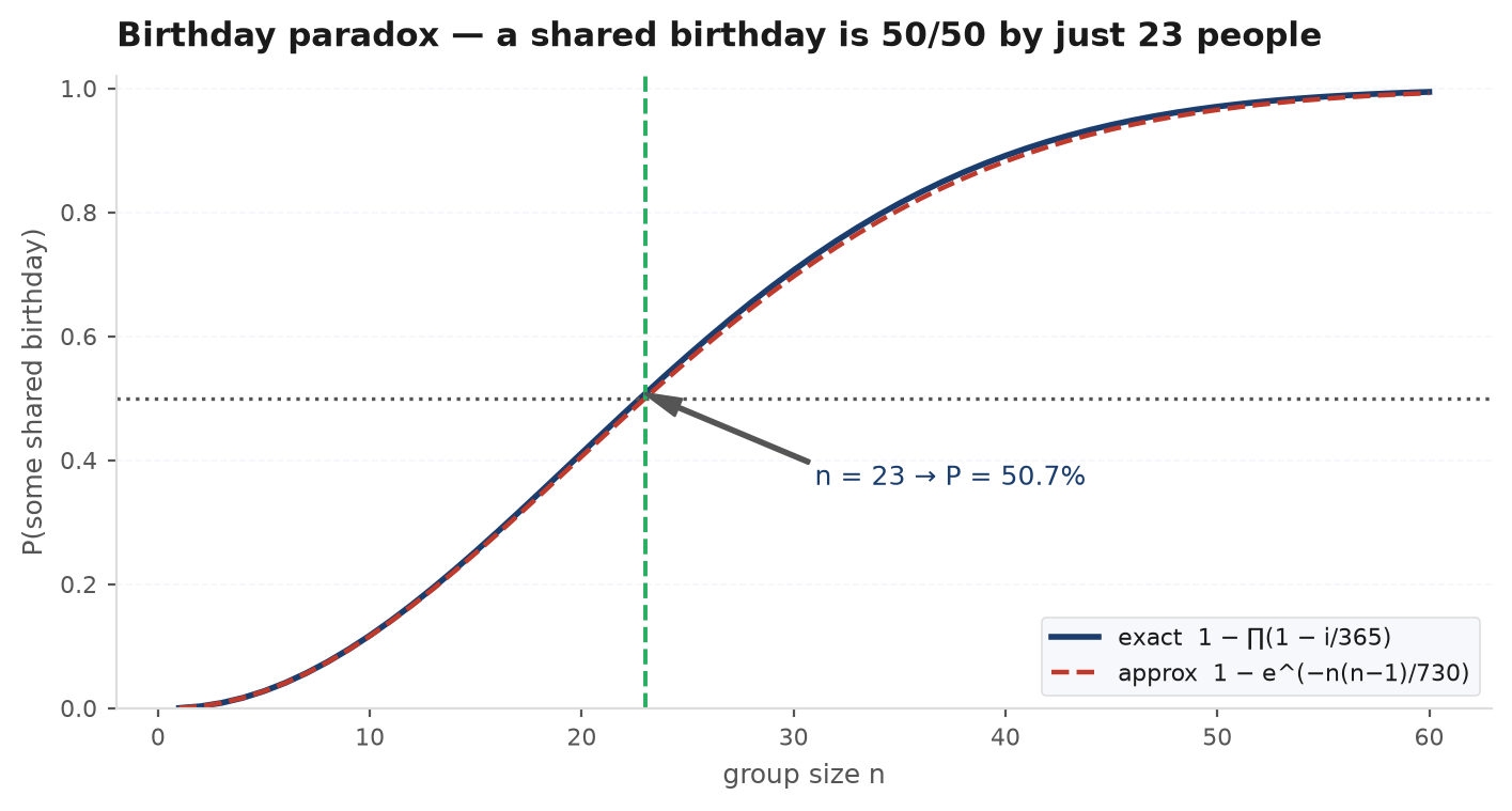
The basic computation — 23 people suffice for a 50% chance of a shared birthday — is worked in counting & combinatorics. Here we explain the scaling, because the exact number 23 is a consequence of a law worth far more than it. With $m$ balls and $n$ bins,

P (no collision) = k = 1 \prod m - 1 (1 - \frac{k}{n}) \approx exp (- k = 1 \sum m - 1 \frac{k}{n}) = exp (- \frac{m ( m - 1 )}{2 n}),

using $1 - x \approx e^{- x}$ for small $x$ . The exponent is the expected number of colliding pairs, and that is no coincidence:

✦Proof — expected colliding pairs, by indicators

For each of the $(2 m)$ pairs of balls, let $X_{ij} = 1 {balls i, j share a bin}$ . Whatever bin ball $i$ chose, ball $j$ matches it with probability $1/ n$ , so $E [X_{ij}] = 1/ n$ . Linearity — dependence between pairs be damned — gives

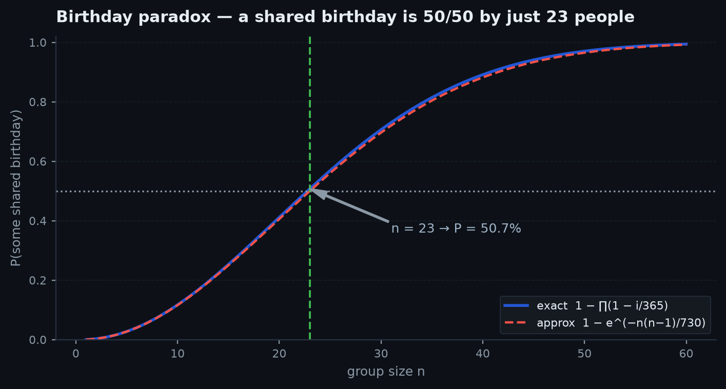
E [# colliding pairs] = (2 m) \frac{1}{n} = \frac{m ( m - 1 )}{2 n} . ■

Collisions become likely precisely when this expectation reaches order 1 — i.e. when $m \approx 2 n ln 2 \approx 1.18 n$ , the solution of $e^{- m^{2} /2 n} = \frac{1}{2}$ . For $n = 365$ : $2 \cdot 365 ln 2 \approx 22.5$ , and indeed 23 people give collision probability $0.507$ . Check the exponent: at $m = 23$ the expected pair count is $\frac{23 \cdot 22}{730} = 0.693 \approx ln 2$ — the 50% threshold is exactly where the expected number of collisions hits $ln 2$ .

The moral: collisions appear at $n$ , not $n$ , because pairs grow quadratically in $m$ . Nobody needs to hit your birthday (that takes $\approx 253$ people for a 50% chance); someone only needs to hit someone’s, and there are $(2 23) = 253$ chances among 23 people. The same quadratic is the birthday attack in cryptography: finding some pair of inputs with the same hash — enough to forge a signature — takes only $\approx 2^{b /2}$ attempts against a $b$ -bit hash, not $2^{b}$ . A 64-bit hash resists a preimage hunt at $2^{64}$ but folds to a collision hunt at $2^{32} \approx 4 \times 1 0^{9}$ — an afternoon of computation. This is why cryptographic hashes are 256 bits: the security level is half the width.

Probability that at least two people in a group share a birthday as group size grows, crossing 50 percent at 23 people — The birthday curve: collision probability against group size, crossing 1/2 at m = 23 ≈ √(2·365·ln 2). The rise is one minus a Gaussian in m — glacial at first, then decisive — because the exponent m(m−1)/730 is the expected number of colliding pairs and grows quadratically.

Empty bins and the 37% law#

Now ask the opposite question: which bins receive nothing? Let $E_{i} = 1 {bin i empty}$ . Each ball misses bin $i$ with probability $1 - 1/ n$ , independently, so $E [E_{i}] = (1 - 1/ n)^{m}$ , and linearity gives

E [# empty bins] = n (1 - \frac{1}{n})^{m} ⟶ n e^{- m / n} .

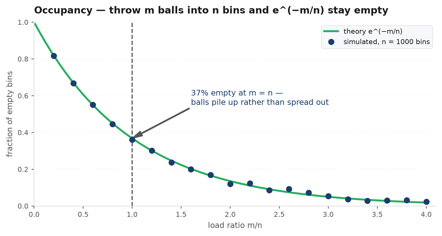
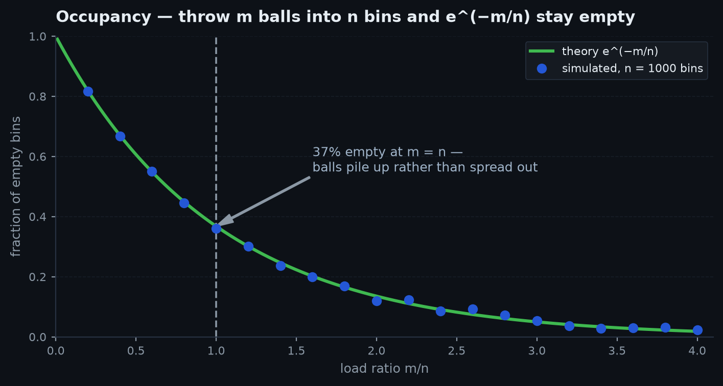
At $m = n$ — as many balls as bins — the empty fraction is $(1 - 1/ n)^{n} \to e^{- 1} \approx 36.8%$ . Uniform randomness is far lumpier than intuition expects: throw 365 balls at 365 days and about 134 days receive no ball, which forces other days to double and triple up — the empty-bin law and the birthday paradox are two faces of the same clumping. (This $1 - e^{- 1} \approx 63.2%$ coverage number is the same one that says a bootstrap resample touches about 63% of the original data points — resampling & bootstrap.)

✦Proof sketch — the empty count concentrates

Is the fraction actually close to $e^{- m / n}$ , or only on average? Compute the variance. With $Z = \sum_{i} E_{i}$ ,

Var (Z) = n (1 - \frac{1}{n})^{m} + n (n - 1) (1 - \frac{2}{n})^{m} - n^{2} (1 - \frac{1}{n})^{2 m},

since two bins are both empty iff every ball avoids both: $E [E_{i} E_{j}] = (1 - 2/ n)^{m}$ . Because $(1 - 2/ n)^{m} < (1 - 1/ n)^{2 m}$ , the covariances are negative — one bin being empty leaves more balls to fill the others — and a short expansion shows $Var (Z) = O (n)$ while $E [Z] = Θ (n)$ . Chebyshev then pins the empty fraction within $O (n^{- 1/2})$ of $e^{- m / n}$ with high probability. ■ The simulation below finds the fraction within a third of a percent of $1/ e$ already at $n = 1 0^{5}$ .

Simulated fraction of empty bins as the ball-to-bin ratio m over n grows, lying on top of the exponential curve e to the minus m over n — The empty-bin law: simulated fraction of empty bins against the load ratio m/n, sitting on the curve e^{−m/n}. At m = n a full 37% of bins are untouched; doubling the balls to m = 2n still leaves 13.5% empty. Uniform allocation does not spread evenly — it clumps, and this curve prices the clumping.

Poissonisation: pretending the bins are independent#

Bin loads are dependent, but barely. The marginal is $Binomial (m, 1/ n)$ , and by the law of rare events (common distributions) — many trials, tiny success probability — this converges to $Poisson (λ)$ with $λ = m / n$ :

P (L_{i} = k) = (k m) (\frac{1}{n})^{k} (1 - \frac{1}{n})^{m - k} ⟶ e^{- λ} \frac{λ ^{k}}{k !} .

The stronger — and more useful — statement is the Poissonisation heuristic: the joint vector of loads behaves like $n$ independent $Poisson (m / n)$ variables. Why is that legitimate? If you throw a $Poisson (m)$ number of balls instead of exactly $m$ , the thinning property of Poisson processes (Poisson processes) makes the loads exactly independent $Poisson (m / n)$ — and a Poisson( $m$ ) count is $m \pm O (m)$ , a vanishing relative difference — a standard transfer lemma makes the comparison precise at the cost of an $O (m)$ factor on probabilities. Sanity checks it passes instantly: expected empty bins $= n P (Poisson (λ) = 0) = n e^{- λ}$ (matches), expected singleton bins $= nλ e^{- λ}$ , expected doubly-occupied days $= n \frac{λ ^{2}}{2} e^{- λ}$ (Problem 2 tests this against the exact count).

!When Poissonisation lies

The heuristic is trustworthy for bulk statistics — counts of bins with a given load, fractions, maxima — up to the $O (m)$ transfer cost. It fails for statements that feel the exact total: the true loads sum to $m$ always, Poisson loads only on average, so “the sum of all loads” has variance 0 in reality and $m$ under Poissonisation. Never use it on a quantity pinned by the constraint.

Maximum load, and the power of two choices#

Throw $n$ balls into $n$ bins — average load exactly 1. How bad is the worst bin? The answer is one of the most quoted results in randomised algorithms:

i max L_{i} = Θ (\frac{lo g n}{lo g lo g n}) with high probability.

✦Proof sketch — union bound on overloaded bins

Fix a bin and a level $k$ . The chance the bin receives at least $k$ named balls is at most $(k n) (1/ n)^{k} \leq (\frac{e n}{k})^{k} n^{- k} = (e / k)^{k}$ (choose which $k$ balls, demand each land there, ignore the rest — an over-count, hence an upper bound). Union over all $n$ bins (inequalities & bounds):

P (i max L_{i} \geq k) \leq n (\frac{e}{k})^{k} .

Take $k = 3 ln n / ln ln n$ : then $(e / k)^{k} = e^{- k (l n k - 1)} \approx e^{- 3 l n n} = n^{- 3}$ , since $ln k \approx ln ln n$ . The bound becomes $n^{- 2} \to 0$ . A matching lower bound (via Poissonisation: the chance no bin among $n$ near-independent Poisson(1) loads reaches $k$ dies once $n \cdot \frac{e ^{- 1}}{k !} ≫ 1$ ) shows the order is exact. ■ The rate comes from $k! \approx n$ : factorials beat exponentials, so the max load grows slower than $lo g n$ — about 4–5 for $n = 1 0^{4}$ , only 8 or so for $n = 1 0^{5}$ , as the simulation confirms.

Now the miracle. Change the protocol: for each ball, pick two bins uniformly at random and place the ball in the emptier of the two. The maximum load collapses to

\frac{ln ln n}{ln 2} + O (1) \approx 3.5 at n = 1 0^{5} — doubly exponentially better.

Why one extra glance is worth so much. For a bin to climb to height $k + 1$ under two choices, a ball must draw two bins that are both already at height $\geq k$ . If a fraction $β_{k}$ of bins reach height $k$ , the chance of that double-draw is $β_{k}^{2}$ — so the fractions square at every level: $β_{k + 1} \approx β_{k}^{2}$ , giving $β_{k} \approx 2^{- 2^{k}}$ — doubly exponential decay, hence a maximum at $lo g_{2} lo g n$ ; with one choice the decay is only factorial. This is why real load balancers sample two servers and route to the shorter queue — nearly all the benefit of full information, at the price of two random probes.

The coupon collector as occupancy#

Final question: how many balls until no bin is empty? That is the coupon collector — each cereal box a ball, each coupon type a bin, collection complete when every bin is hit. The stage decomposition (expectation & linearity, brainteasers) does expectation in three lines: when $i - 1$ bins are occupied, each throw hits a new bin with probability $(n - i + 1) / n$ , so the wait for the $i$ -th new bin is geometric with mean $n / (n - i + 1)$ , and

E [T] = i = 1 \sum n \frac{n}{n - i + 1} = n (\frac{1}{1} + \frac{1}{2} + \dots + \frac{1}{n}) = n H_{n} \approx n ln n + 0.577 n .

The occupancy view explains the $n ln n$ : after $m$ throws the expected number of still-empty bins is $n e^{- m / n}$ , which passes through 1 exactly at $m = n ln n$ . The last few coupons cost almost everything — the first half of the bins fill in $n ln 2 \approx 0.69 n$ throws, while the final lone bin alone costs $n$ throws on average.

Around $n ln n$ the transition is sharp. Writing $m = n ln n + c n$ , the expected empty count is $n e^{- m / n} = e^{- c}$ , and by Poissonisation the number of empty bins is approximately Poisson with that mean, so

P (T \leq n ln n + c n) ⟶ exp (- e^{- c}),

the Gumbel distribution — the same double-exponential law that governs the maximum of i.i.d. exponentials in order statistics, and no accident: $T$ is the maximumover bins of each bin’s first-hit time, and maxima of light-tailed waiting times are Gumbel territory. The fluctuations of $T$ around $n ln n$ are only $O (n)$ — relatively tiny — which is why “have I sampled every state?” questions flip from almost-certainly-no to almost-certainly-yes over a narrow window.

Non-uniform bins only make collisions worse#

Real birthdays are not uniform — September peaks, holidays dip. Does that break the 23-person answer? It strengthens it. Let bin $i$ receive each ball with probability $p_{i}$ . Two independent balls collide with probability

P (pair collides) = i = 1 \sum n p_{i}^{2} \geq \frac{1}{n}, with equality iff p_{i} \equiv 1/ n .

✦Proof — Jensen in one line, and the general statement

$\sum_{i} p_{i}^{2} = n \cdot \frac{1}{n} \sum_{i} p_{i}^{2} \geq n (\frac{1}{n} \sum_{i} p_{i})^{2} = n \cdot \frac{1}{n ^{2}} = \frac{1}{n}$ by Jensen’s inequality (inequalities & bounds) applied to the convex function $x \mapsto x^{2}$ : the average of squares beats the square of the average, strictly unless all $p_{i}$ are equal. ■ The per-pair statement lifts to the full event: for every group size $m$ , the no-collision probability $m! \sum_{i_{1} < \dots < i_{m}} p_{i_{1}} \dots p_{i_{m}}$ is a Schur-concave function of $(p_{1}, \dots, p_{n})$ — maximised at the uniform distribution, so any non-uniformity can only raise the collision probability. Intuitively: skew concentrates balls in the popular bins, and collisions live where the mass piles up.

So the textbook 23 is conservative: with real birthday frequencies the 50% point arrives at 23 or earlier, never later. The same convexity works against you in hashing — a hash function with a biased output distribution collides faster than the uniform analysis promises, by exactly the factor $n \sum_{i} p_{i}^{2}$ — and in any bucketing scheme where the traffic is skewed: collision risk is priced by $\sum p_{i}^{2}$ (the “collision entropy”), not by the bin count $n$ .

→Quant lens — occupancy is market plumbing

Bucketing trades into time bins is the occupancy model verbatim: $m$ fills spread over $n$ one-minute bars leaves $\approx e^{- m / n}$ of bars empty even if arrivals are perfectly uniform — so sparse bars are not evidence of regime change, and any per-bar statistic must budget for the 37% law before reading meaning into gaps (Poisson processes is the continuous-time version). Hash-based deduplication of market data feeds is a birthday problem: dedupe $1 0^{6}$ messages through a 32-bit fingerprint and the expected number of false merges is $(2 1 0 ^{6}) / 2^{32} \approx 116$ — silently dropped ticks; Problem 5 sizes the table properly. And when a desk runs 30 strategies that each fire in a handful of regime-bins, the birthday arithmetic says some pair will “collide” — crowd onto the same trade in the same hour — far sooner than intuition expects, with the rate inflated by $n \sum p_{i}^{2}$ because everyone’s signal fires in the same high-vol bins. Correlated books built from “independent” strategies are a non-uniform birthday problem you are on the wrong side of.

Simulation: all four laws at once#

One experiment checks everything: throw $n$ balls into $n$ bins, then read off the empty fraction, the colliding pairs, and the maximum load — plus the two-choice variant to watch the max load collapse.

occupancy_laws.py

import numpy as np

rng = np.random.default_rng(21)

print(f"{'n':>7} | empty frac (1/e=0.3679) | coll. pairs (theory) | max load")
for n in [100, 1_000, 10_000, 100_000]:
    counts = np.bincount(rng.integers(0, n, n), minlength=n)  # m = n balls
    empty = (counts == 0).mean()
    pairs = (counts * (counts - 1) // 2).sum()   # sum of C(load, 2)
    print(f"{n:>7} | {empty:.4f}                  | "
          f"{pairs:>6} ({(n - 1) / 2:>8.1f})    | {counts.max()}")

# Power of two choices: place each ball in the emptier of two random bins.
n = 100_000
counts = np.zeros(n, dtype=int)
a, b = rng.integers(0, n, n), rng.integers(0, n, n)
for i in range(n):
    j = a[i] if counts[a[i]] <= counts[b[i]] else b[i]
    counts[j] += 1
print(f"two-choice max load at n={n}: {counts.max()} "
      f"(theory ~ lnln n/ln 2 = {np.log(np.log(n)) / np.log(2):.1f}; "
      f"one-choice gave 8)")

Representative output: empty fractions 0.3600, 0.3660, 0.3652, 0.3678 marching to $1/ e = 0.3679$ ; colliding pairs within a few percent of $(n - 1) /2$ ; one-choice max loads 4, 5, 6, 8 against a two-choice max load of 4 even at $n = 1 0^{5}$ .

Practice problems#

Five problems that test whether the occupancy picture is actually installed — each is a balls-into-bins question in disguise, and each yields to indicators, the exponential approximation, or Poissonisation.

→Problem 1 — sharing a birth week

How many people are needed for a 50% chance that two share a birth week (52 equally likely weeks)?

Solution. The scaling law answers first: $m \approx 2 \cdot 52 ln 2 = 72.1 \approx 8.5$ , so guess 9. Exactly: $P (all distinct) = \prod_{k = 1}^{m - 1} (1 - k /52)$ , which is $0.568$ at $m = 8$ (collision 43.2%) and $0.480$ at $m = 9$ (collision 52.0%). Answer: 9 people. Note the ratio to the day version: $23/9 \approx 2.6 \approx 365/52 = 7$ — shrinking the bins sevenfold shrinks the threshold by $7$ , exactly the $n$ law. If you remember one thing, remember that collisions scale with the square root of the bin count.

→Problem 2 — days that are exactly two people's birthday

In a group of 50 people (365 uniform days), what is the expected number of calendar days that are the birthday of exactly two people?

Solution. Indicator per bin: day $i$ has exactly two birthdays with probability $(2 50) (1/365)^{2} (364/365)^{48}$ , so the expectation is $365 (2 50) \frac{1}{36 5 ^{2}} (364/365)^{48} = \frac{1225}{365} (0.8766) \approx 2.94$ days. Poissonisation gets the same number faster: each day’s count is approximately $Poisson (λ)$ with $λ = 50/365 = 0.137$ , so the answer is $365 \cdot e^{- λ} λ^{2} /2 \approx 2.99$ — within 1.5% of exact. Meanwhile the same group has $365 λ e^{- λ} \approx 43.7$ singleton days and $365 e^{- λ} \approx 318$ empty days. Lesson: for “how many bins have load $k$ ” questions, linearity plus the Poisson profile $n e^{- λ} λ^{k} / k!$ is the whole method.

→Problem 3 — rolling a die until every face appears

Roll a fair die until every face has appeared at least once. Compute the expected number of rolls exactly.

Solution. Coupon collector with $n = 6$ bins. Stage decomposition: with $i - 1$ faces seen, the wait for a new face is geometric with success probability $(7 - i) /6$ , mean $6/ (7 - i)$ . Sum:

E [T] = 6 (\frac{1}{1} + \frac{1}{2} + \frac{1}{3} + \frac{1}{4} + \frac{1}{5} + \frac{1}{6}) = 6 \cdot \frac{49}{20} = \frac{147}{10} = 14.7.

The stage breakdown is the insight: the first three new faces cost $1 + 1.2 + 1.5 = 3.7$ rolls, the last face alone costs 6. Against the continuous approximation $n ln n + 0.577 n = 14.2$ — close even at $n = 6$ . Lesson: expectations decompose over stages even though the stages are dependent in every other respect; linearity does not care.

→Problem 4 — one empty bin, and the independence illusion

Throw $m$ balls into $n$ bins. What is the probability that bin 1 stays empty? Are the events “bin 1 empty” and “bin 2 empty” independent?

Solution. Each ball misses bin 1 with probability $1 - 1/ n$ independently, so $P (bin 1 empty) = (1 - 1/ n)^{m} \approx e^{- m / n}$ . For the pair: $P (both empty) = (1 - 2/ n)^{m}$ , while independence would demand $(1 - 1/ n)^{2 m}$ . Since $1 - \frac{2}{n} < (1 - \frac{1}{n})^{2} = 1 - \frac{2}{n} + \frac{1}{n ^{2}}$ , the joint probability is strictly smaller: the events are negatively correlated — balls that spare bin 1 are recycled toward bin 2. But the gap is $O (m / n^{2})$ in the exponent, vanishing for large $n$ : asymptotically the bins decouple — the Poissonisation heuristic seen from below. Lesson: bins are never independent, only almost independent, and knowing the size of “almost” is what separates using the heuristic from being used by it.

→Problem 5 — sizing a hash table for a million keys

You must hash $1 0^{6}$ keys with probability less than 1% that any two collide. How large must the hash space $n$ be? Does a 64-bit hash suffice?

Solution. Collision probability $\approx 1 - e^{- m^{2} /2 n} < 0.01$ requires $\frac{m ^{2}}{2 n} < - ln 0.99 \approx 0.01005$ , i.e. $n > \frac{1 0 ^{12}}{0.0201} \approx 5.0 \times 1 0^{13} \approx 2^{45.5}$ . So 46 bits of hash are needed for a million keys at the 1% level — the quadratic pair count means the hash space must scale with the square of the key count. A 64-bit hash gives $P (collision) \approx \frac{m ^{2}}{2 \cdot 2 ^{64}} = \frac{1 0 ^{12}}{3.7 \times 1 0 ^{19}} \approx 2.7 \times 1 0^{- 8}$ — comfortable; a 32-bit hash gives expected $\frac{m ( m - 1 )}{2 \cdot 2 ^{32}} \approx 116$ collisions — a certainty of silent data corruption. Lesson: for collision safety, budget bits at $2 lo g_{2} m$ plus a safety margin, never $lo g_{2} m$ — the birthday attack arithmetic, now working for you.

Next: the occupancy model rewards careful conditioning — and the next chapter is a gallery of problems where careless conditioning produces confident, wrong answers: Simpson reversals, the two envelopes, and friends. Probability paradoxes.