Symmetry & exchangeability

The deepest skill in probability is getting the answer without computing anything. This chapter builds the two tools that make it possible: the symmetry principle — a measure-preserving relabelling of outcomes forces two events to have equal probability — and exchangeability, the statement that a random sequence does not care about order. Together they answer questions that look like they need conditional-probability marathons (“what is the chance the 17th card is an ace?”) in one line, and they are the exact hypothesis behind permutation tests. The principle is proved once, then used relentlessly: card positions, relative orders, gaps, random permutations, rotations around a circle, and sampling without replacement.

✦Intuition — if the mechanism can't tell two events apart, neither can the probability

Probability is assigned by a mechanism — a shuffle, a sequence of flips, a uniform draw. If you can exhibit a relabelling of outcomes that the mechanism is blind to (swapping two cards before a uniform shuffle changes nothing) and that relabelling carries event $A$ onto event $B$ , then $P (A) = P (B)$ — no counting required. The entire art is choosing what to ignore: to compare two cards, ignore the other fifty; to locate the first ace, ignore the identities of the non-aces; to test a trading signal, ignore the labels the null hypothesis says are arbitrary. Every result below is one application of this move, and the discipline that keeps it honest is always the same — name the map, check it preserves the measure.

The symmetry principle#

Let $φ : Ω \to Ω$ be a bijection of outcomes that preserves probabilities: $P (φ (E)) = P (E)$ for every event $E$ . If $φ$ maps $A$ onto $B$ , then

P (A) = P (φ (A)) = P (B) .

That is the whole theorem — one line, directly from the definition. For a finite space with equally likely outcomes every bijection preserves probabilities, which is why shuffled decks are such fertile ground: any relabelling of the 52 cards, applied before a uniform shuffle, leaves the distribution over orderings untouched. The principle also delivers equalities of distributions, not just of single probabilities: if $X \circ φ = Y$ for a measure-preserving $φ$ , then $X$ and $Y$ have the same distribution, hence the same mean, variance, everything.

✦Worked example — a first taste: heads before tails

Flip a fair coin 100 times. What is the probability that flips 1–50 contain more heads than flips 51–100 contain tails? Apply the map that flips every coin in the second half only — fair independent flips make it measure-preserving, and it turns second-half tails into second-half heads. So the question equals $P (H_{1 : 50} > H_{51 : 100})$ , and the further symmetry that exchanges the two halves makes that $\frac{1}{2} (1 - P (tie))$ . No binomial sums — two relabellings peeled the problem down to its genuinely asymmetric core, a tie probability.

Exchangeability: order-blindness made precise#

A finite or infinite sequence $X_{1}, X_{2}, \dots$ is exchangeable if every reordering has the same joint distribution: for each $n$ and every permutation $π$ of ${1, \dots, n}$ ,

(X_{π (1)}, \dots, X_{π (n)}) = d (X_{1}, \dots, X_{n}) .

Two consequences do most of the work in practice: all marginals agree (each $X_{i}$ has the distribution of $X_{1}$ ), and all pairs agree ( $(X_{i}, X_{j}) = d (X_{1}, X_{2})$ for $i \neq = j$ , so every pair shares one covariance). Exchangeable variables need not be independent — that is the entire point:

i.i.d. ⟹ exchangeable. The joint law of an i.i.d. vector is a product of identical factors, and products do not care about the order of their factors.
Exchangeable ⟹̸ i.i.d. Deal cards from a shuffled deck without replacement. Every ordering of the 52 cards is equally likely, so any relabelling of positions is measure-preserving: the sequence of dealt cards is exchangeable. But it is glaringly dependent — if the first card is the ace of spades, the second cannot be.

✦Proof — dealing without replacement is exchangeable

A uniform shuffle assigns probability $1/52!$ to every ordering. Fix a permutation $π$ of positions and consider the map $φ$ sending the ordering $ω$ to the ordering whose $i$ -th card is $ω_{π (i)}$ — a bijection of the $52!$ equally likely outcomes, hence measure-preserving, with $(X_{π (1)}, \dots, X_{π (52)}) (ω) = (X_{1}, \dots, X_{52}) (φ (ω))$ by construction. Equal distributions follow from the symmetry principle. ■ Nothing about card values, suits, or how many cards you deal was used: any function of a uniformly random permutation inherits this order-blindness.

Every position of a shuffled deck is a uniform draw#

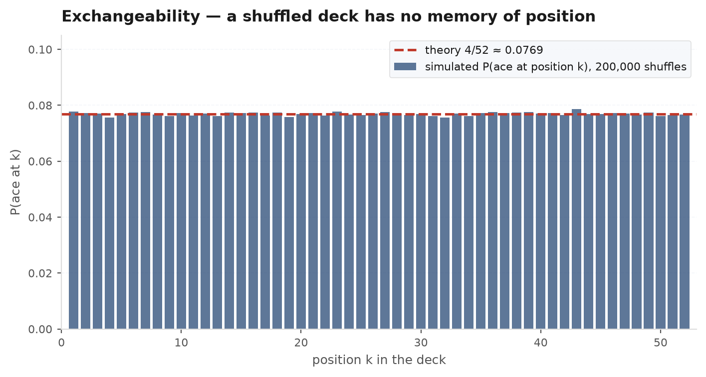
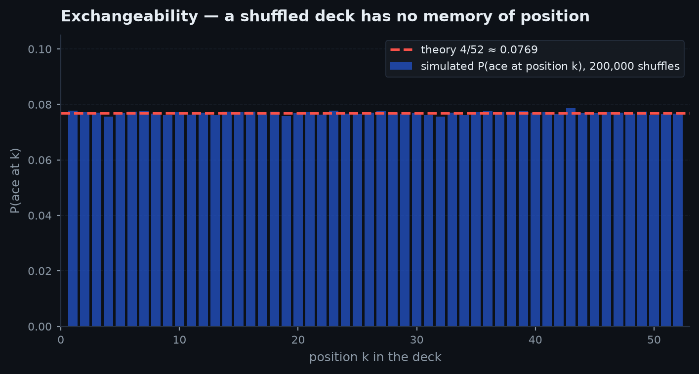
The marginal-equality consequence, spelled out for cards: in a shuffled deck, the card at position $k$ is a uniform draw from the 52 cards, for every $k$ . So

P (17th card is an ace) = P (1st card is an ace) = \frac{4}{52} = \frac{1}{13} \approx 7.69%.

The instinct that resists this — “surely it depends on what the first sixteen cards were” — confuses a conditional probability with a marginal one. Had you seencards 1–16, the probability would update (to $(4 - a) /36$ after observing $a$ aces). But unseen cards reveal nothing: no information has arrived, so there is nothing to condition on, and position 17 is exactly as ignorant as position 1. The formal one-liner: the transposition swapping positions 1 and 17 before a uniform shuffle is measure-preserving and maps “ace at 17” onto “ace at 1.” The same argument makes the last card a uniform draw — hard enough to believe that it is worth simulating.

Simulated probability that each position 1 through 52 of a shuffled deck holds an ace, flat at 4/52 across all positions with the theoretical line overlaid — The deck has no memory of position: the simulated probability that position k holds an ace sits at 4/52 ≈ 7.69% for every k from 1 to 52, within Monte Carlo noise of the theory line. Exchangeability makes every position marginally identical — as true for position 52 as for position 1, however counterintuitive that feels before you name the swap map.

Relative order: condition on the subset, use uniformity#

Question: in a shuffled deck, what is $P (card i comes before card j)$ ? Answer: $1/2$ , by the transposition that swaps the two cards before shuffling — it is measure-preserving and exchanges the events “ $i$ first” and “ $j$ first,” which are complementary. The general and far more powerful statement:

✦Proof sketch — the relative order of any subset is uniform

Fix any subset $S$ of $m$ cards. Condition on which positions the cards of $S$ occupy. Given those positions, every assignment of the $m$ cards to them is equally likely — any of the $m!$ permutations of $S$ is a measure-preserving relabelling that fixes the positions and permutes the assignment. So the relative order of $S$ is uniform over $m!$ orderings, independently of where the rest of the deck put them. ■

This is the tool that makes irrelevant clutter vanish. Is the ace of spades more likely than the ace of hearts to appear first in a deck that also contains two jokers, or a hundred? Irrelevant — restrict to the two-card subset: uniform over its $2!$ orderings, so $1/2$ whatever else is in the deck. Probability the ace of spades precedes both red aces: uniform over $3! = 6$ orderings of those three cards, first in 2 of them: $1/3$ . All four aces before all four kings: $4! \times 4!$ of $8!$ orderings, i.e. $1/ (4 8) = 1/70$ (Problem 5 works this in full). The counting techniques of counting & combinatorics still matter — but only after symmetry has shrunk the problem to the subset that actually varies.

Gaps: where is the first ace?#

The 4 aces cut the other 48 cards into 5 gaps: before the first ace, three gaps between consecutive aces, and after the last. How large is the first gap on average? Symmetry again — this time on each non-ace separately. Fix a particular non-ace card and restrict to the 5-card subset consisting of it and the four aces: its relative order among them is uniform over 5 slots, so it lands before all four aces with probability exactly $1/5$ . By linearity of expectation over indicator variables (expectation & linearity),

E [cards before the first ace] = 48 \times \frac{1}{5} = \frac{48}{5} = 9.6,

so the expected position of the first ace is $\frac{48}{5} + 1 = \frac{53}{5} = 10.6$ . The same argument gives each of the five gaps expected size $48/5$ — the gaps are exchangeable, another distribution shared by relabelling. The general result, for $k$ special cards among $n$ :

E [position of first special card] = \frac{n - k}{k + 1} + 1 = \frac{n + 1}{k + 1} .

Sanity checks: $k = n$ gives position 1; $k = 1$ gives $(n + 1) /2$ , the centre — a single special card is uniform over positions, as it must be. For the deck: 10.6 for the first ace, $53/14 \approx 3.79$ for the first heart. The continuous twin — $k$ uniform points cutting $[0, 1]$ into $k + 1$ exchangeable spacings of mean $1/ (k + 1)$ — is developed in order statistics.

deck_symmetry_checks.py

import numpy as np

rng = np.random.default_rng(17)
trials = 200_000

# Only the ace / non-ace pattern matters: cards 0-3 are the aces.
ranks = np.argsort(rng.random((trials, 52)), axis=1)  # each row: a uniform shuffle
is_ace = ranks < 4

# Expected position of the first ace (1-indexed): theory (n+1)/(k+1) = 53/5
first_ace = is_ace.argmax(axis=1) + 1
print(f"E[position of first ace] = {first_ace.mean():.3f}   (theory 53/5 = 10.600)")

# P(17th card is an ace): theory 4/52 = 1/13
p17 = is_ace[:, 16].mean()
print(f"P(17th card is an ace)   = {p17:.4f}   (theory 1/13 = 0.0769)")

# Exchangeability across ALL positions: the per-position ace frequency is flat
freq = is_ace.mean(axis=0)  # the deck has no memory: flat across positions
print(f"per-position ace freq: min={freq.min():.4f}  max={freq.max():.4f}  "
      f"(all approx 0.0769)")

Random permutations: positions, cycles, and Hₙ#

A uniformly random permutation $π$ of ${1, \dots, n}$ is the shuffled deck in abstract clothing, and symmetry reads off its structure:

Each element is uniform over positions: $P (π (i) = j) = 1/ n$ for all $i, j$ — compose with a transposition of targets, exactly the ace-at-position-17 argument.
Cycle lengths are uniform too: the cycle containing any fixed element has length $L$ with $P (L = ℓ) = 1/ n$ for every $ℓ = 1, \dots, n$ — a flat distribution, which few people guess.

✦Proof sketch — the cycle containing element 1 has uniform length

Follow the cycle: $1 \to π (1) \to π (π (1)) \to \dots$ . At the first step, $π (1)$ is uniform over $n$ values, so the cycle closes immediately with probability $1/ n$ . Given it did not, the next value is uniform over the $n - 1$ remaining, closing with probability $1/ (n - 1)$ . Multiplying survival and closing probabilities telescopes:

P (L = ℓ) = \frac{n - 1}{n} \cdot \frac{n - 2}{n - 1} \dots \frac{n - ℓ + 1}{n - ℓ + 2} \cdot \frac{1}{n - ℓ + 1} = \frac{1}{n} . ■

The same telescoping pattern — survival probabilities cancelling against the next denominator — appears in the birthday-problem and hat-check calculations of counting & combinatorics.

The uniform cycle length buys the expected number of cycles for free. Each element $i$ sits in a cycle of length $L_{i}$ , and a cycle of length $ℓ$ is counted once by each of its $ℓ$ members if we weight each member by $1/ L_{i}$ . So the cycle count is $\sum_{i} 1/ L_{i}$ , and by linearity plus the flat law of $L_{i}$ :

E [# cycles] = i = 1 \sum n E [\frac{1}{L _{i}}] = n ℓ = 1 \sum n \frac{1}{ℓ} \cdot \frac{1}{n} = H_{n} = 1 + \frac{1}{2} + \dots + \frac{1}{n} \approx ln n .

For $n = 52$ : $H_{52} \approx 4.54$ cycles on average. Decompositions of this flavour are the subject of expectation & linearity; here symmetry supplied the marginal law that linearity then summed.

Rotations: the cycle lemma and round tables#

Transpositions are not the only useful symmetry. Rotations power the slickest proof of the ballot theorem. Candidate A gets $a$ votes, B gets $b < a$ , counted in uniformly random order; the claim is

P (A strictly leads throughout the count) = \frac{a - b}{a + b} .

✦Proof sketch — the cycle lemma

Encode votes as $+ 1$ (A) and $- 1$ (B) and bend the sequence of $n = a + b$ votes into a circle. The cycle lemma (Dvoretzky–Motzkin): for any circular arrangement with total sum $k = a - b > 0$ , exactly $k$ of the $n$ starting points give all partial sums strictly positive — they are the steps just after each of the $k$ distinct record minima of the running sum. Now the symmetry: a uniformly random ordering makes all $n$ rotations of any circular arrangement equally likely — rotation is a measure-preserving bijection — so the probability of an always-positive count is $k / n = (a - b) / (a + b)$ , whichever circular arrangement you were dealt. ■ With $a = 60, b = 40$ : only $20%$ — even a landslide winner usually gets caught at least once. The reflection-principle proof of the same fact lives in random walks & Brownian motion.

The everyday version of rotation symmetry is the round table. Seat $n$ people uniformly at random around a circle; what is the probability two particular friends sit together? Rotate so that friend one’s seat is fixed — rotations are measure-preserving, so this loses nothing. The other $n - 1$ seats are now exchangeable for friend two, and 2 of them are adjacent: $P = 2/ (n - 1)$ , i.e. $2/9 \approx 22.2%$ at a table of 10. The “fix one person by rotation” move dissolves nearly every circular-arrangement problem — the line version appears as Problem 4.

Sampling without replacement: exchangeability at work in statistics#

Draw $n$ values $X_{1}, \dots, X_{n}$ without replacement from a population of $N$ numbers with mean $μ$ and variance $σ^{2}$ . The draws are dependent — but exchangeable, by the dealing argument above. Exchangeability alone gives:

Unbiasedness for free: each $X_{i}$ is marginally a uniform draw from the population, so $E [X_{i}] = μ$ and $E [X ˉ] = μ$ . The sample mean is unbiased regardless of the dependence.
Negative correlation: drawing a large value removes it from the pool, tilting later draws small. Quantitatively, $Cov (X_{i}, X_{j}) = - σ^{2} / (N - 1)$ for $i \neq = j$ .

✦Proof — the covariance, pinned by a degenerate case

By exchangeability all pairs $(X_{i}, X_{j})$ , $i \neq = j$ , share one covariance $c$ — so a single clever case determines it. Take $n = N$ : the sample is the whole population, so $\sum_{i = 1}^{N} X_{i}$ is a constant with variance zero. Expanding,

0 = Var (i = 1 \sum N X_{i}) = N σ^{2} + N (N - 1) c ⟹ c = - \frac{σ ^{2}}{N - 1} . ■

Feeding $c$ into the variance of a mean of $n$ exchangeable draws gives

Var (X ˉ) = \frac{σ ^{2}}{n} \frac{N - n}{N - 1},

the finite population correction: sampling without replacement is more accurate than i.i.d. sampling, because each draw genuinely retires part of the uncertainty — at $n = N$ the variance hits zero, a census. The estimator-level consequences are developed in estimators & sampling.

→Quant lens — exchangeability is the permutation-test licence

A permutation test asks: shuffle the labels (long/short days, strategy A/B trades, regime tags) and recompute the statistic — is the observed value extreme among the shuffles? The logic is precisely this chapter’s: under the null hypothesis the labelled sequence is exchangeable, so every relabelling is measure-preserving and the observed arrangement is a uniform draw from the shuffled ensemble — making the permutation p-value exact, with no normality and no asymptotics. The licence is also the limitation: autocorrelated or volatility-clustered returns are not exchangeable, so naive shuffling destroys real structure and overstates significance — the reason block permutations exist. The machinery is built in resampling & the bootstrap: when you shuffle a backtest’s trade labels, you are asserting exchangeability — make sure the null you care about actually implies it (why backtests lie).

!“It feels symmetric” is not an argument

Every result above named an explicit measure-preserving map: a transposition, a rotation, a relabelling. That discipline is the difference between a proof and a trap. Bertrand’s paradoxis the canonical failure: “choose a random chord of a circle; what is the probability it is longer than the side of the inscribed equilateral triangle?” Three natural symmetries — random endpoints, random midpoint, random distance from the centre — give $1/3$ , $1/4$ , and $1/2$ . All three feel symmetric; they are symmetric under different groups, and “random chord” never specified the generating mechanism. The paradox dissolves the moment the mechanism is named — the full dissection lives in geometric probability. The working rule: a symmetry argument is complete only when you state the bijection, check it preserves the measure of the actual mechanism, and exhibit it mapping one event onto the other.

Practice problems#

Five problems that test whether the reflex is installed — each collapses under a single well-chosen symmetry, and each solution names its map.

→Problem 1 — the last card

A standard deck is shuffled. What is the probability that the last card is a spade?

Solution.The transposition swapping positions 1 and 52 before the shuffle is measure-preserving and maps “spade at 52” onto “spade at 1,” so the answer is the first-card answer: $13/52 = 1/4$ . No conditioning on the first 51 cards, because none were observed — unseen cards carry no information. The one-line insight: every unobserved position of a shuffled deck is marginally a uniform draw; position 52 is not special.

→Problem 2 — waiting for the first heart

Turn cards over one at a time from a shuffled deck. What is the expected number of cards you turn over until the first heart appears (counting the heart itself)?

Solution. The 13 hearts cut the 39 non-hearts into 14 exchangeable gaps. For each non-heart, restrict to the 14-card subset of it plus the 13 hearts: its relative order is uniform, so it precedes all 13 hearts with probability $1/14$ . Linearity: $E [non-hearts before first heart] = 39/14$ , so the expected count including the heart is $39/14 + 1 = 53/14 \approx 3.79$ — the general $(n + 1) / (k + 1)$ with $n = 52, k = 13$ . The one-line insight: don’t track the deck card by card — drop each irrelevant card into the gaps and let uniform relative order price it.

→Problem 3 — cutting for high card

You and an opponent each reveal one card from the same shuffled deck; higher rank wins, and equal ranks are a tie. What is the probability you win outright — and given the cut is not a tie, what is the probability it was broken in your favour?

Solution.The map that swaps the two revealed cards is measure-preserving and exchanges “you higher” with “opponent higher,” so those probabilities are equal, and given no tie your win probability is exactly $1/2$ — symmetry settles the conditional before any counting. Only the tie needs arithmetic: given your card, 3 of the remaining 51 cards match its rank, so $P (tie) = 3/51 = 1/17$ and $P (win outright) = \frac{1}{2} (1 - \frac{1}{17}) = 8/17 \approx 47.1%$ . The one-line insight: symmetry splits the non-tie mass exactly in half; computation is only ever needed for the part the symmetry doesn’t reach.

→Problem 4 — your two friends adjacent in line

$n$ people, including your two friends, line up in uniformly random order. What is the probability your friends end up adjacent?

Solution. The pair of positions occupied by the two friends is uniform over all $(2 n)$ unordered pairs — permuting the other people is measure-preserving and washes them out. Adjacent pairs number $n - 1$ (positions ${1, 2}, {2, 3}, \dots, {n - 1, n}$ ), so

P (adjacent) = \frac{n - 1}{( 2 n )} = \frac{2}{n} .

For $n = 10$ : $1/5$ , slightly below the round table’s $2/ (n - 1)$ — a circle has one extra adjacency. The one-line insight: reduce to the joint law of the positions you care about — everyone else is exchangeable scenery.

→Problem 5 — all aces before all kings

In a shuffled deck, what is the probability that all four aces appear before all four kings?

Solution. Restrict to the eight-card subset of aces and kings: its relative order is uniform over $8!$ orderings, wherever the other 44 cards fall. The event demands the first four of those eight be the aces (in any internal order): $4! \times 4!$ favourable orderings, so

P = \frac{4 ! 4 !}{8 !} = \frac{1}{( 4 8 )} = \frac{1}{70} \approx 1.43%.

Equivalently: which four of the eight relative slots the aces occupy is uniform over $(4 8) = 70$ choices, and exactly one — the first four slots — wins. The one-line insight: the other 44 cards are noise; condition on the subset and the answer is a count over its uniform orderings.

Next: from relabelling outcomes to reshaping distributions — how densities transform under functions of a random variable, the Jacobian formula, and the universality of the uniform. Transformations of random variables.