Transformations of random variables

You rarely get to work with the variable you were given: prices are exponentials of returns, risk is a maximum over desks, a portfolio is a sum. This chapter builds the complete toolkit for finding the distribution of $Y = g (X)$ — the CDF method as universal fallback, the change-of-variables formula and its Jacobian, convolutions for sums, product CDFs for extremes, and the probability integral transform that turns uniform noise into any distribution you like. The recurring picture is conservation of mass: a transformation moves probability around without creating or destroying it, and every formula here is an accounting identity for where the mass went.

✦Intuition — probability is mass; a transformation is a flow

Picture the distribution of $X$ as a unit of sand spread along the line with local thickness $f_{X}$ . The map $g$ picks up every grain at $x$ and drops it at $g (x)$ : no sand is created or lost, but compression piles the same sand higher and stretching thins it out. Every formula in this chapter — the Jacobian factor, the convolution integral, the chi-square density blowing up at zero — is this one picture written in calculus. When in doubt, forget densities entirely and track the mass directly through the CDF: that method never fails.

The CDF method: the universal fallback#

To find the distribution of $Y = g (X)$ , compute $F_{Y} (y) = P (g (X) \leq y)$ by expressing the event ${g (X) \leq y}$ as a set of $x$ -values, reading its probability off $F_{X}$ , and differentiating. This works for any $g$ — monotone or not — because it manipulates probabilities (honest numbers) rather than densities (rates). Every fancier formula below is a shortcut through this computation.

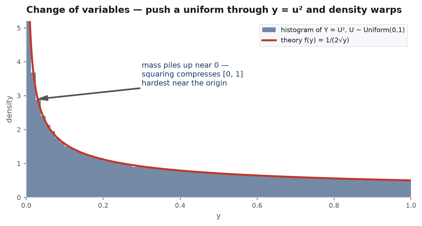
✦Worked example — Y = X² for a uniform, and for a normal

Uniform. Let $U \sim Unif (0, 1)$ , $Y = U^{2}$ . For $y \in (0, 1)$ , $F_{Y} (y) = P (U^{2} \leq y) = P (U \leq y) = y$ , so

f_{Y} (y) = \frac{d}{d y} y = \frac{1}{2 y}, 0 < y < 1.

The density is unbounded near 0 — more on why in a moment — yet integrates to 1: $\int_{0}^{1} \frac{1}{2 y} d y = 1$ ; and since $F_{Y} (1/4) = 1/2$ , half the mass lands below $1/4$ .

Normal. Let $X \sim N (0, 1)$ , $Y = X^{2}$ . Now the map is two-to-one, and the CDF method handles it without blinking: $F_{Y} (y) = P (- y \leq X \leq y) = 2Φ (y) - 1$ for $y > 0$ . Differentiating with the chain rule,

f_{Y} (y) = 2 φ (y) \cdot \frac{1}{2 y} = \frac{1}{2 π y} e^{- y /2}, y > 0.

This is the chi-square distribution with 1 degree of freedom — the building block of every variance estimate. Both densities blow up at 0 for the same reason: squaring compresses the whole neighbourhood of $x = 0$ (where the parent density is largest) into a tiny sliver near $y = 0$ , and the sand piles up.

Change of variables: the Jacobian factor#

When $g$ is strictly monotone and differentiable, the CDF method can be run once and packaged as a formula. For increasing $g$ , $F_{Y} (y) = F_{X} (g^{- 1} (y))$ and the chain rule differentiates it; for decreasing $g$ a minus sign appears, and the absolute value covers both cases:

f_{Y} (y) = f_{X} (g^{- 1} (y)) \frac{d g ^{- 1} ( y )}{d y} .

Read the factor $∣ d g^{- 1} / d y ∣$ as a local exchange rate between lengths: a small interval $[y, y + d y]$ of output is the image of an input interval of length $∣ d g^{- 1} / d y ∣ d y$ , whose mass is exactly what lands on $[y, y + d y]$ . Equate that mass to $f_{Y} (y) d y$ , cancel the $d y$ , and the formula appears. Where the map stretches, the same mass covers more ground and the density is diluted; where it compresses, the density is concentrated.

!Density is not probability

A density carries units: probability per unit length of $y$ . Measure a waiting time in seconds instead of hours and the density changes by a factor of 3600 while every actual probability stays fixed. That is why densities can exceed 1 (the $1/ (2 y)$ above is 5 at $y = 0.01$ ) and even diverge, and why $f_{Y} (y) \neq = f_{X} (g^{- 1} (y))$ : forgetting the Jacobian silently asserts that the map neither stretches nor compresses anything — true only for shifts. Probabilities are invariant under the flow; densities are not.

Histogram of Y equals U squared for U uniform on (0,1), with the theoretical density one over two root y overlaid, showing density diverging near zero — Mass conservation under squaring: the histogram of Y = U² matches the theoretical density 1/(2√y), which diverges at 0. The map compresses the input interval (0,1) hardest near 0 — the whole stretch of u-values below 0.1 lands in (0, 0.01) — so the same probability mass occupies less room and the density piles up. Mass is conserved; density is not.

✦Worked example — linear maps, and a scale check

For $Y = a X + b$ : $g^{- 1} (y) = (y - b) / a$ , Jacobian $1/∣ a ∣$ , so $f_{Y} (y) = \frac{1}{∣ a ∣} f_{X} (\frac{y - b}{a})$ . This is why the $N (μ, σ^{2})$ density carries a $1/ σ$ out front, and why an $Exp (λ)$ density is $λ e^{- λ y}$ : stretching a standard exponential by $1/ λ$ dilutes its density by the same factor. Sanity-check every transformation against the linear case — a formula that gets $a X$ wrong is missing its Jacobian.

Log and exp: the lognormal#

The most important nonlinear map in finance is the exponential. If $X \sim N (μ, σ^{2})$ and $Y = e^{X}$ , then $g^{- 1} (y) = ln y$ with Jacobian $1/ y$ , and the change-of-variables formula gives the lognormal density

f_{Y} (y) = \frac{1}{y σ 2 π} exp (- \frac{( ln y - μ ) ^{2}}{2 σ ^{2}}), y > 0.

Asset prices are modelled lognormal for a structural reason: prices compound multiplicatively, so the log price is a sum of many small log returns, approximately normal by the CLT (LLN & CLT). Exponentiating yields a lognormal price — automatically positive, skewed right, fat upper tail. The applied consequences of working in logs are developed in returns & compounding.

!The mean of a lognormal is NOT e^μ

The median of $Y = e^{X}$ is $e^{μ}$ — monotone maps carry quantiles across exactly. The mean is strictly larger:

E [e^{X}] = e^{μ + σ^{2} /2} > e^{μ} = e^{E [X]} .

The convex function $e^{x}$ amplifies upside deviations more than it damps downside ones, so averaging after the map beats mapping the average — a first sighting of Jensen’s inequality, proved properly in inequalities & bounds. With $σ = 0.2$ (an ordinary annual equity vol) the factor is $e^{0.02} \approx 1.020$ — a 2% gap between mean and median, every year, from curvature alone.

→Quant lens — volatility drag is a change of variables

A strategy whose log return has mean $μ$ and variance $σ^{2}$ per period grows wealth at median rate $e^{μ}$ but expected rate $e^{μ + σ^{2} /2}$ ; equivalently, a simple return with mean $m$ compounds at roughly $m - σ^{2} /2$ in log terms. That $σ^{2} /2$ is volatility drag: two strategies with identical average returns but different vols end at different wealth, and the arithmetic-mean backtest column overstates what you will compound — the median outcome, not the mean, is what a single account experiences (position sizing). When a backtest metric and your account balance disagree, suspect a transformation applied on the wrong side of the expectation.

Min and max: extremes via CDFs#

For extremes of independent variables the CDF method is the natural tool, because max and min turn into intersections of independent events:

P (i max X_{i} \leq x) = i = 1 \prod n F_{i} (x), P (i min X_{i} > x) = i = 1 \prod n (1 - F_{i} (x)) .

The maximum is small only if everyone is small; the minimum is large only if everyone is large. For i.i.d. variables these become $F (x)^{n}$ and $1 - (1 - F (x))^{n}$ . The full machinery of ranked values — every intermediate rank, not just the two ends — is the subject of order statistics.

✦Worked example — the minimum of exponentials is exponential

Let $X_{i} \sim Exp (λ_{i})$ be independent, so $P (X_{i} > x) = e^{- λ_{i} x}$ . Then

P (i min X_{i} > x) = i \prod e^{- λ_{i} x} = e^{- (λ_{1} + \dots + λ_{n}) x},

so $min_{i} X_{i} \sim Exp (λ_{1} + \dots + λ_{n})$ : exponential with the summed rates. Servers failing at rates 1, 2, and 3 per year produce a first failure at rate 6 — expected wait two months; moreover $P (X_{j} is the minimum) = λ_{j} / \sum_{i} λ_{i}$ . This pair of facts is the engine room of Poisson processes: merging independent streams adds their rates because the next arrival is a minimum of exponential waits.

Sums: convolution#

For independent $X$ and $Y$ , the density of $S = X + Y$ is the convolution

f_{S} (s) = \int_{- \infty}^{\infty} f_{X} (x) f_{Y} (s - x) d x, P (S = s) = x \sum P (X = x) P (Y = s - x) (discrete) .

Read it as a sweep over the ways to land on $s$ : whatever the first variable contributes, the second must supply exactly the rest, and independence multiplies the densities. The discrete version is how two dice make 7 more often than 12 — more ways to split it.

✦Derivation — the triangle density of two uniforms

Let $U_{1}, U_{2} \sim Unif (0, 1)$ independent, $S = U_{1} + U_{2} \in (0, 2)$ . The integrand $f_{U_{1}} (x) f_{U_{2}} (s - x)$ equals 1 exactly on the overlap of $(0, 1)$ and $(s - 1, s)$ , so the density of $S$ is the length of that overlap:

f_{S} (s) = {s, 2 - s, 0 \leq s \leq 1, 1 \leq s \leq 2.

A triangle peaking at 1: slide a unit window across a unit block and record the overlap — maximal when centred, shrinking linearly toward the ends. There are simply more ways to make 1 than to make 0.1 (both variables must be tiny). Add a third uniform and the density turns piecewise quadratic and bell-ish; add thirty and it is visually indistinguishable from a normal — convolution smooths, and iterated convolution is the CLT in the making (LLN & CLT).

One closure fact to keep loaded — normal + normal = normal: for independent $X \sim N (μ_{1}, σ_{1}^{2})$ and $Y \sim N (μ_{2}, σ_{2}^{2})$ , $X + Y \sim N (μ_{1} + μ_{2}, σ_{1}^{2} + σ_{2}^{2})$ . Grinding the convolution integral proves it, but the civilised route is through transforms: generating functionsturn convolution into multiplication — whenever a convolution integral looks painful, that chapter’s machinery is the shortcut.

Ratios: the Cauchy distribution#

Let $X, Y \sim N (0, 1)$ be independent and $Z = X / Y$ . Given $Y = y$ , $Z = X / y$ has density $∣ y ∣ φ (z y)$ (the linear-map rule again); averaging over $y$ :

f_{Z} (z) = \int_{- \infty}^{\infty} ∣ y ∣ φ (z y) φ (y) d y = \frac{1}{2 π} \int_{- \infty}^{\infty} ∣ y ∣ e^{- (1 + z^{2}) y^{2} /2} d y = \frac{1}{π ( 1 + z ^{2} )} .

(The last integral is elementary after substituting $t = y^{2}$ .) This is the Cauchy distribution — bell-shaped near the centre, pathological in the tails: $f_{Z} (z) \sim 1/ (π z^{2})$ , so $\int ∣ z ∣ f_{Z} (z) d z$ diverges and the Cauchy has no mean — not a large mean, no mean. The mechanism is visible in the construction: the denominator spends real time near zero, and dividing by a near-zero produces occasional enormous outputs.

The consequence for averages is brutal: if $Z_{1}, \dots, Z_{n}$ are i.i.d. Cauchy, their sample mean is exactly Cauchy again— averaging a million observations leaves you precisely as uncertain as one. The LLN’s hypothesis $E ∣ Z ∣ < \infty$ fails and its conclusion fails with it, the canonical fat-tail failure dissected in LLN & CLT. Any pipeline that averages ratios of noisy quantities — hedge ratios from short windows, statistics with tiny denominators — is flirting with this regime, and the symptom is sample means that never settle down.

The probability integral transform#

One transformation is so useful it gets its own name. Let $X$ have a continuous, strictly increasing CDF $F$ :

Forward: $F (X) \sim Unif (0, 1)$ — any continuous variable, pushed through its own CDF, becomes uniform.
Backward: if $U \sim Unif (0, 1)$ , then $F^{- 1} (U) \sim F$ — a uniform, pushed through any inverse CDF, acquires that distribution.

✦Proof — both directions in two lines

Forward: for $u \in (0, 1)$ , $P (F (X) \leq u) = P (X \leq F^{- 1} (u)) = F (F^{- 1} (u)) = u$ — the uniform CDF. Backward: $P (F^{- 1} (U) \leq x) = P (U \leq F (x)) = F (x)$ . ■ Both lines are one move — $F$ is monotone, so applying it to both sides of an inequality preserves the event. Intuitively, $F (X)$ is the rank of $X$ within its own distribution, and your rank in your own distribution is uniform by construction.

The backward direction is inverse-transform sampling, the foundation of simulation: a generator that only produces uniforms can produce anything with a computable inverse CDF — for the exponential, $F^{- 1} (u) = - ln (1 - u) / λ$ , verified in code below. This is how Monte Carlo methodsmanufacture their raw material; the forward direction is how models are audited (a correct model’s CDF applied to real data must be uniform), and why order statistics of any continuous distribution reduce to those of uniforms (order statistics) — rank first, transform later.

Several variables at once: the multivariate Jacobian#

The one-dimensional formula generalises verbatim, the derivative promoted to a determinant: if $g : R^{n} \to R^{n}$ is a differentiable bijection and $Y = g (X)$ , then

f_{Y} (y) = f_{X} (g^{- 1} (y)) det J_{g^{- 1}} (y),

where $J_{g^{- 1}}$ is the matrix of partial derivatives of the inverse map. The determinant is the volume exchange rate: a small box $d y$ of output pulls back to a parallelepiped of volume $∣ det J ∣ d y$ , and mass conservation does the rest — the same sand-pile argument, one dimension up.

✦Worked example — Box-Muller: two uniforms in, two normals out

Let $U_{1}, U_{2} \sim Unif (0, 1)$ be independent and set

Z_{1} = - 2 ln U_{1} cos (2 π U_{2}), Z_{2} = - 2 ln U_{1} sin (2 π U_{2}) .

Claim: $Z_{1}, Z_{2}$ are independent standard normals. Sketch: the joint density of two standard normals, $\frac{1}{2 π} e^{- (z_{1}^{2} + z_{2}^{2}) /2}$ , becomes in polar coordinates (area element $r d r d θ$ , Jacobian $r$ ) the product $(\frac{1}{2 π} d θ) (r e^{- r^{2} /2} d r)$ : a uniform angle, independent of a radius whose square is $Exp (1/2)$ . Box-Muller builds exactly that pair from two uniforms — $Θ = 2 π U_{2}$ is the uniform angle, and $R^{2} = - 2 ln U_{1}$ is $Exp (1/2)$ by inverse-transform sampling — then converts back to Cartesian. ■ Note the miracle: the outputs share one $R$ and one $Θ$ yet come out independent — a rotational-symmetry fingerprint unique to the Gaussian, and a workhorse of Monte Carlo methods.

Simulation check: triangle density and inverse-transform sampling#

Two claims verified numerically: the triangle density, and inverse-transform exponentials vs numpy.

transform_checks.py

import numpy as np

rng = np.random.default_rng(23)
n = 1_000_000

# --- 1. Triangle density of U1 + U2 ---------------------------------
s = rng.random(n) + rng.random(n)
tri = lambda x: np.where(x <= 1, x, 2 - x)          # theoretical density
for lo, hi in [(0.4, 0.5), (0.95, 1.05), (1.7, 1.8)]:
    emp = np.mean((s >= lo) & (s < hi)) / (hi - lo)  # empirical density
    mid = (lo + hi) / 2
    print(f"density near s={mid:.2f}:  empirical {emp:.4f}   theory {tri(mid):.4f}")

# --- 2. Inverse-transform exponential vs numpy's exponential --------
lam = 1.5
u = rng.random(n)
x_inv = -np.log(1 - u) / lam          # F^{-1}(U) = -ln(1-U)/lambda
x_np  = rng.exponential(1 / lam, n)   # numpy's own sampler

print(f"\nmean:   inverse {x_inv.mean():.4f}   numpy {x_np.mean():.4f}   theory {1/lam:.4f}")
print(f"var:    inverse {x_inv.var():.4f}   numpy {x_np.var():.4f}   theory {1/lam**2:.4f}")
for q in [0.5, 0.95]:
    th = -np.log(1 - q) / lam
    print(f"q={q}:  inverse {np.quantile(x_inv, q):.4f}   "
          f"numpy {np.quantile(x_np, q):.4f}   theory {th:.4f}")
# The two samplers agree to Monte Carlo error: F^{-1}(U) IS the exponential.

Practice problems#

Five problems testing whether the mass-conservation picture is really installed — each a one-transformation question with a standard trap.

→Problem 1 — the reciprocal of a uniform

$X \sim Unif (1, 2)$ , $Y = 1/ X$ . Find the density of $Y$ and check it integrates to 1.

Solution. $Y$ lives on $(1/2, 1)$ . CDF method with a decreasing map: $F_{Y} (y) = P (1/ X \leq y) = P (X \geq 1/ y) = 2 - 1/ y$ , using $F_{X} (x) = x - 1$ . Differentiate: $f_{Y} (y) = 1/ y^{2}$ on $(1/2, 1)$ . Check: $\int_{1/2}^{1} y^{- 2} d y = [- 1/ y]_{1/2}^{1} = - 1 + 2 = 1$ . ✓ The density is 4 at $y = 1/2$ and 1 at $y = 1$ : inversion compresses the far end of $(1, 2)$ into a sliver near $1/2$ , so mass piles up there. The naive answer “uniform on $(1/2, 1)$ ” is the missing-Jacobian error: nonlinear maps do not preserve uniformity.

→Problem 2 — the maximum of n uniforms

$U_{1}, \dots, U_{n} \sim Unif (0, 1)$ i.i.d., $M = max_{i} U_{i}$ . Find the distribution of $M$ and its expectation.

Solution. Product of CDFs: $F_{M} (x) = P (all U_{i} \leq x) = x^{n}$ on $(0, 1)$ , so $f_{M} (x) = n x^{n - 1}$ , piling up against 1 as $n$ grows. Expectation: $E [M] = \int_{0}^{1} n x^{n} d x = \frac{n}{n + 1}$ — with $n = 9$ , $0.9$ ; with $n = 99$ , $0.99$ ; the gap to 1 shrinks like $1/ (n + 1)$ . The best backtest among $n$ random strategies behaves the same way — the running maximum drifts up mechanically, edge or no edge, the selection-bias engine quantified in multiple testing & paradoxes.

→Problem 3 — the half-normal

$X \sim N (0, 1)$ , $Y = ∣ X ∣$ . Find the density and mean of $Y$ .

Solution. The map is two-to-one, so use the CDF: for $y > 0$ , $F_{Y} (y) = P (- y \leq X \leq y) = 2Φ (y) - 1$ , giving $f_{Y} (y) = 2 φ (y) = 2/ π e^{- y^{2} /2}$ — the half-normal: the two symmetric branches of mass fold onto one side and the density doubles. Mean: $E ∣ X ∣ = 2 \int_{0}^{\infty} y φ (y) d y = 2 φ (0) = 2/ π \approx 0.798$ , since the integrand is $- φ^{'} (y)$ . Takeaway: mean absolute deviation $\approx 0.8 σ$ for Gaussians — a quick fat-tail diagnostic when the observed ratio drifts from 0.8.

→Problem 4 — sum of two exponentials, by convolution

$X, Y \sim Exp (λ)$ independent. Find the density of $S = X + Y$ by convolution.

Solution. Both densities vanish on negatives, so the integral runs over $(0, s)$ :

f_{S} (s) = \int_{0}^{s} λ e^{- λ x} λ e^{- λ (s - x)} d x = λ^{2} e^{- λ s} \int_{0}^{s} d x = λ^{2} s e^{- λ s}, s > 0.

The integrand is constant because the exponents recombine into $e^{- λ s}$ whatever the split — every division of the total wait is equally likely. The result is the Gamma $(2, λ)$ density: zero at 0 (two waits are rarely both tiny), peak at $s = 1/ λ$ ; iterating gives Gamma $(n, λ)$ — the arrival times of a Poisson process.

→Problem 5 — build a density from a uniform

Given $U \sim Unif (0, 1)$ , construct a random variable with density $f (x) = 2 x$ on $(0, 1)$ .

Solution. Inverse transform. The target CDF is $F (x) = \int_{0}^{x} 2 t d t = x^{2}$ , whose inverse is $F^{- 1} (u) = u$ . So $X = U$ does it — check directly: $P (U \leq x) = P (U \leq x^{2}) = x^{2}$ . ✓ A pleasing duality with the chapter’s opening example: squaring a uniform piles mass toward 0; square-rooting piles it toward 1 — and $U$ is also the distribution of $max (U_{1}, U_{2})$ from Problem 2. Lesson: if you can write the CDF and invert it, you can simulate the distribution — no rejection, no special functions, one line of code.

Next: convolution integrals were the hard way — transforms turn sums into products and distributional identities into algebra: Generating functions.