Probability paradoxes

A paradox is a precise confusion: two arguments that both look airtight and contradict each other. None of the classics in this chapter is a genuine contradiction — each is a theorem plus a mis-stated model, and locating the mis-statement is the entire exercise. Dissected properly, every one of them leaves a permanent upgrade: St. Petersburg teaches you what expectation cannot do, the two envelopes teach you what a prior is for, the boy–girl family teaches you that how information arrived matters as much as what it says, and non-transitive dice teach you that pairwise comparisons refuse to aggregate. This capstone stress-tests everything Part II built, at the exact points where intuition snaps.

✦Intuition — a paradox is an under-specified experiment

Every paradox below dissolves the same way: write down the experiment— the full generating procedure, including how the information you hold was produced — and compute inside that model, because the contradiction always lives in the gap between two different experiments wearing the same words. “The other envelope holds double or half” is not a model until you say what distribution the amounts came from; “at least one child is a boy” is not evidence until you say how you learned it. And the fallback is mechanical: simulate the procedure and let frequencies arbitrate.

St. Petersburg: infinite expectation, twenty-dollar offers#

Flip a fair coin until the first head. If the head arrives on toss $k$ , you are paid $2^{k}$ . The expected payout is

E [X] = k = 1 \sum \infty 2^{- k} \cdot 2^{k} = 1 + 1 + 1 + \dots = \infty.

So an expectation-maximiser should pay any finite price to play — yet almost nobody pays more than about $20. The instinct is right, in three distinct ways worth separating.

Bounded bankrolls truncate the sum. A counterparty who can pay at most $2^{30}$ (about a billion) caps the series at 30 terms: $E [X \land 2^{30}] = 30 + 1 = 31$ (thirty $1 terms plus the capped tail — Problem 1). The truncated game is worth roughly $lo g_{2} (bankroll)$ : the “infinite” value is supplied entirely by payouts no real counterparty can honour.
The typical outcome is tiny. The median payout is 2 and $P (X \leq 8) = 7/8$ . The mean is dragged to infinity by outcomes you will essentially never see; the mean–median gap is the whole story. A log-utility player computes $E [lo g_{2} X] = \sum_{k} k 2^{- k} = 2$ , a certainty equivalent of $2^{2} = 4$ — Bernoulli’s original 1738 resolution.
The sample mean never settles. Because $E [X] = \infty$ , the law of large numbers (LLN & CLT) does not apply — the running mean of $n$ plays grows like $lo g_{2} n$ (Feller: the fair fee for a block of $n$ games is about $n lo g_{2} n$ ). No amount of experience converges to a price, because there is no price to converge to.

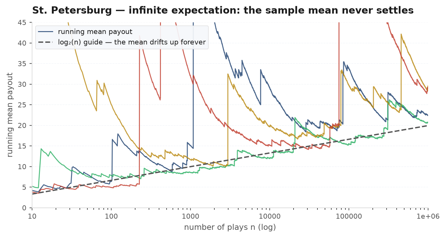
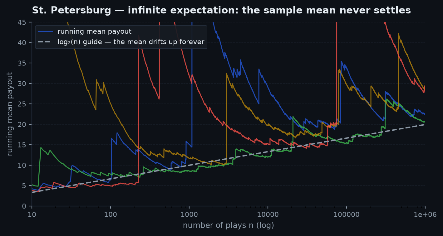
Running sample mean of St. Petersburg payouts over many plays on a logarithmic x-axis for several seeds, climbing without settling and jumping at rare deep runs — Infinite expectation in practice: the running sample mean of St. Petersburg payouts never converges — it lurches upward at every new record payout and climbs like log2(n) between lurches. Each seed tells the same story with different jump times: the rare deep runs that carry the expectation have never all happened yet, and never will have.

→Quant lens — expectation alone cannot price a gamble

St. Petersburg is the cleanest possible model of a fat-tailed strategy: almost all plays return a small amount, and the entire expectation lives in rare monsters. First, sample means of fat-tailed P&L converge glacially or not at all — a short-vol or tail-buying book cannot be judged by its backtest average, because the observations that dominate $E$ are exactly the ones missing from any finite sample (LLN & CLT). Second, a positive — even infinite — expectation says nothing about what to pay or size: sizing is a statement about the whole distribution and your bankroll, which is why the Kelly criterion maximises $E [lo g (wealth)]$ rather than $E [wealth]$ — Bernoulli’s fix, three centuries early (position sizing).

The two-envelope paradox: the prior you forgot to state#

Two envelopes, one holding twice the other. You pick one, see $X = x$ , and are offered a swap. The seductive argument: the other envelope holds $x /2$ or $2 x$ , each with probability $1/2$ , so

E [other ∣ X = x] = \frac{1}{2} \cdot \frac{x}{2} + \frac{1}{2} \cdot 2 x = \frac{5 x}{4} > x — always switch?

Always switching cannot be right by symmetry: before opening anything, the two envelopes are exchangeable, so switching gains exactly zero. The error is a single unstated assumption: “the other is $x /2$ or $2 x$ with probability $1/2$ each, for every observed $x$ ” is a claim about the conditional distribution of the pair given your observation — and no prior on the amounts makes it true. It would require every pair $(2^{k}, 2^{k + 1})$ to be equally likely — a uniform distribution on an infinite set, which no more exists than a uniform distribution on all positive reals. Conditioning on $X = x$ requires a prior over pairs; the paradox smuggles in an improper one and computes with it (conditional expectation, Bayesian inference).

✦Worked example — the correct analysis under a proper prior

Give the pair a real distribution: $(10, 20)$ with probability $p$ , $(20, 40)$ with probability $1 - p$ ; pick an envelope uniformly. Observe $x = 20$ — the only ambiguous value. Both pairs produce a 20 with likelihood $1/2$ , so the posterior over pairs equals the prior, and

E [other ∣ X = 20] = p \cdot 10 + (1 - p) \cdot 40 = 40 - 30 p .

Switch iff $40 - 30 p > 20$ , i.e. iff $p < 2/3$ . Seeing 10 you always switch; seeing 40 you never do. That is the general shape under any proper prior: switching is right below a thresholdand wrong above it, because a large observed amount is itself evidence that you already hold the bigger envelope. Averaged over everything, gains and losses cancel exactly — symmetry restored, paradox gone. An expectation conditional on data is only defined relative to a prior, and “I have no prior” is not a prior.

Boy–girl, Tuesday’s boy, and the procedure that produced the words#

The boy–girl puzzles were solved by counting in axioms, conditioning & Bayes: “at least one of two children is a boy” gives $P (both boys) = 1/3$ ; “at least one is a boy born on a Tuesday” gives $13/27$ . The general lesson those answers were hiding: the probability depends on the procedure that produced the information, not on the information alone. Compare two ways of learning the same sentence:

“She told me at least one is a boy.” If this report is guaranteed whenever the family has any boy, it merely deletes $GG$ from ${B B, B G, GB, GG}$ : answer $1/3$ .
“I met one of her children — a boy.”Now the evidence is “a uniformly random child of the family is a boy.” Likelihoods: $P (evidence ∣ B B) = 1$ but $P (evidence ∣ B G) = P (evidence ∣ GB) = 1/2$ . Posterior odds for $B B$ against “one of each”: $1 \cdot \frac{1}{4} : \frac{1}{2} \cdot \frac{1}{2} = 1 : 1$ — answer $1/2$ .

Same sentence, different experiments, different answers. The Tuesday-boy jump from $1/3$ toward $1/2$ is the same phenomenon in motion: the more specific the reported feature, the more the report behaves like pointing at a particular child, which gives $1/2$ . This is exactly Monty Hall’s protocol-dependence: the host who must open a goat door and the host who happened to open one produce different likelihood ratios from the identical visible event. Condition on the mechanism, not the words.

!Pitfall — treating a report as a random sample

The failure mode in the wild: treating volunteered information as a neutral sample. A fund that tells you about its best strategy, a backtest you chose to look at because it looked good — the reporting rule is part of the experiment, and ignoring it is how selection bias enters (multiple testing & paradoxes). “At least one of my strategies has a Sharpe above 2” differs from “this randomly audited strategy has a Sharpe above 2” for precisely the boy–girl reason.

Bertrand’s box and the three prisoners: Monty Hall in disguise#

Three boxes: one holds two gold coins, one two silver, one one of each. Pick a box at random, draw a coin at random: it is gold. What is the chance the other coin in your box is also gold? The reflex answer $1/2$ ignores that the GG box is twice as good at producing the evidence; the odds form (Bayes) settles it in three lines:

posterior odds \frac{P ( GG ∣ gold )}{P ( GS ∣ gold )} = 1 \frac{1/3}{1/3} \times = \frac{1}{1/2} = 2 \frac{P ( gold ∣ GG )}{P ( gold ∣ GS )} = 2 : 1 ⟹ P (GG ∣ gold) = \frac{2}{3} .

The three prisoners problem is the same computation in a prison uniform: prisoner A, one of three candidates for pardon, asks the warden to name one of the otherswho will be executed; the warden says B. A’s survival probability stays $1/3$ while C’s jumps to $2/3$ — the warden was forced to say B when C holds the pardon but only choseB (coin toss) when A holds it: likelihood ratio 2. Bertrand’s box, the three prisoners, and Monty Hall are one problem — a constrained revealer whose choice leaks information through the constraint. Ask what the revealer could not have shown you, and the likelihood ratio writes itself.

Simpson’s paradox: aggregation reverses conditionals#

It is perfectly possible that $P (W ∣ A, C_{i}) > P (W ∣ B, C_{i})$ in every stratum $C_{i}$ , and yet $P (W ∣ A) < P (W ∣ B)$ overall. No axiom is violated: by the law of total probability, the aggregate is a weighted average of the conditionals, and the two strategies can carry wildly different weights. A compact trading example — win rates across two regimes:

Strategy A: trending regime $8/10 = 80%$ , choppy regime $30/90 = 33.3%$ — overall $38/100 = 38%$ .
Strategy B: trending regime $70/90 = 77.8%$ , choppy regime $3/10 = 30%$ — overall $73/100 = 73%$ .

A beats B in bothregimes (80% vs 77.8%, 33.3% vs 30%) and loses the aggregate by 35 points, because A took 90% of its trades in the hostile regime while B concentrated where winning is easy. Which table answers your question depends on what you control: if you can choose when to trade, per-regime rates matter; if the strategy’s regime mix is intrinsic to it, the aggregate is the honest number. The statistics-flavoured treatment — kidney stones, admissions data, the causal reading — lives in multiple testing & paradoxes; the probability content is just this: aggregation hides conditioning, and a marginal inequality never implies the conditional ones, nor conversely.

Non-transitive dice: “beats” is not an ordering#

Three dice with faces (each value appearing twice):

A = {2, 4, 9}, B = {1, 6, 8}, C = {3, 5, 7} .

Roll two against each other; higher face wins (no ties are possible — the values are distinct). Counting the $3 \times 3 = 9$ equally likely value pairs (each standing for 4 of the 36 face outcomes):

A vs B: A wins on $(2, 1), (4, 1), (9, 1), (9, 6), (9, 8)$ — 5 of 9, so $P (A > B) = 5/9 = 20/36 \approx 0.556$ .
B vs C: B wins on $(6, 3), (6, 5), (8, 3), (8, 5), (8, 7)$ — again $P (B > C) = 5/9$ .
C vs A: C wins on $(3, 2), (5, 2), (5, 4), (7, 2), (7, 4)$ — again $P (C > A) = 5/9$ .

So A beats B beats C beats A, each with probability $5/9$ — a perfect cycle (the magic-square dice; Efron’s four-dice set cycles at $2/3$ ). Nothing is broken: “beats” compares the joint distribution of a pair, and pairwise comparisons of joint distributions have no obligation to chain — transitivity is a property of numbers (means, medians, any scalar summary), not of head-to-head records. Hence the classic hustle: let your opponent pick a die first, then take the one behind it in the cycle.

→Quant lens — pairwise comparisons don't aggregate

Strategy comparisons inherit the disease. “A outperformed B in most months, and B outperformed C in most months” does not imply A outperforms C in most months — month-by-month head-to-heads compare joint distributions, exactly like the dice. Tournament-style rankings built from pairwise records (fund shortlists, model bake-offs) can cycle, and any ranking extracted from them silently depends on the aggregation rule — Condorcet’s voting impossibility in a backtest. If you need an ordering, rank on a scalar and accept what it ignores; if you need head-to-head behaviour, keep the full matrix.

paradox_sims.py

import numpy as np

rng = np.random.default_rng(7)

# --- St. Petersburg: the sample mean grows like log2(n), forever ---
def st_petersburg(n):
    k = rng.geometric(0.5, size=n)   # toss index of the first head
    return 2.0 ** k                  # payout 2^k

for n in (10**3, 10**5, 10**7):
    x = st_petersburg(n)
    print(f"n={n:>10,}   sample mean = {x.mean():9.2f}   log2(n) = {np.log2(n):5.1f}")
# E[X] = infinity: the sample mean climbs with n and never becomes representative.

# --- Non-transitive dice: A beats B beats C beats A, each 5/9 ---
A = np.array([2, 2, 4, 4, 9, 9])
B = np.array([1, 1, 6, 6, 8, 8])
C = np.array([3, 3, 5, 5, 7, 7])

def beats(x, y, n=300_000):
    return (rng.choice(x, n) > rng.choice(y, n)).mean()

print(f"P(A>B) = {beats(A, B):.4f}   (theory 5/9 = 0.5556)")
print(f"P(B>C) = {beats(B, C):.4f}   (theory 5/9 = 0.5556)")
print(f"P(C>A) = {beats(C, A):.4f}   (theory 5/9 = 0.5556)")
# A cycle: no die is 'best'. Pairwise win rates are not an ordering.

The inspection paradox: sampling by size, not by count#

Buses arrive with headways averaging 10 minutes, yet your average wait exceeds 5 — because you are more likely to land inside a long gap: long gaps cover more of the timeline. Arriving at a uniformly random time samples headways with probability proportional to their length: the headway you experience is size-biased, with mean $E [L^{2}] / E [L] \geq E [L]$ (strict unless headways are deterministic), and your expected wait is half of that. For exponential headways with mean 10, the experienced gap averages 20 and the wait is the full 10 — the memorylessness at the heart of Poisson processes, where this gets its complete treatment. The general phenomenon is everywhere: sampling classes in proportion to their size makes the average experienced class bigger than the average class. Your friends have more friends than you do (you sample people in proportion to their friend count); the average fund performance experienced by dollars differs from that by funds — money concentrates in large funds and arrives after good runs, so dollar-weighted returns trail fund-weighted ones. Whenever a summary statistic depends on who is asking, suspect size-biased sampling.

Sleeping Beauty: a genuinely contested question#

One paradox here is honestly unresolved. Beauty sleeps; a fair coin is flipped. Heads: she is woken once (Monday). Tails: woken twice (Monday and Tuesday), her memory of Monday erased. Waking, she is asked: what is your credence that the coin landed heads? Thirders answer $1/3$ : one awakening in three follows heads, so betting at every awakening, 1/3 is the calibrated price. Halfers answer $1/2$ : the coin was fair and waking was certain either way, so nothing discriminating was learned. Both sides compute correctly; they disagree about what “credence” refers to— a per-awakening betting frequency or a per-experiment one. The arithmetic is trivial and undisputed; the referent of the question is not. This marks the honest boundary of the chapter’s method: each paradox above hid one well-posed question, Sleeping Beauty contains two, and no theorem selects between them — know which kind of dispute you are in before arguing.

The meta-lessons#

Five habits, each extracted from at least two of the paradoxes above:

Name the experiment.Sample space, generating procedure, what is random and what is fixed. The two-envelope argument dies the moment you ask “what is the distribution of the pair?”
How information arrived matters. Identical words from different procedures carry different likelihood ratios: told-a-boy vs met-a-boy, forced host vs lucky host, volunteered backtest vs audited backtest.
Expectation is not value. St. Petersburg has infinite mean, median 2, and a street price near $20 — distributions are priced by utility, bankroll, and tails; the mean is one moment, not a verdict.
Aggregation hides conditioning. Simpson reversals, size-biased averages, dollar- vs fund-weighted returns: every aggregate is a weighted average of conditionals, and the weights can carry the whole conclusion.
When confused, simulate. Every well-posed paradox here yields to twenty lines of numpy, because simulation forces you to specify the procedure — always the missing step. If you cannot write the simulation, you have not yet stated the problem.

Practice problems#

Five practice questions that test whether the dissection stuck — in each, the work is stating the experiment; the computing is easy.

→Problem 1 — pricing truncated St. Petersburg

A casino with a bankroll of $2^{30}$ offers St. Petersburg: payout $2^{k}$ if the first head lands on toss $k$ , capped at $2^{30}$ (thirty straight tails pays the cap). What is the fair price?

Solution. Split at the cap. For $k \leq 30$ each term contributes $2^{- k} \cdot 2^{k} = 1$ : total 30. The cap event — thirty tails — has probability $2^{- 30}$ and pays $2^{30}$ : contribution exactly 1. Fair price: $E [X \land 2^{30}] = 30 + 1 = 31$ . Doubling the bankroll to $2^{31}$ adds exactly $1 — value accrues one dollar per doublingof the guarantor, so the uncapped game’s street price is roughly $lo g_{2}$ of whatever you believe they can pay. Expectation is only as real as the tail that carries it.

→Problem 2 — two envelopes with a stated prior

The pair is $(10, 20)$ with probability $0.7$ and $(20, 40)$ with probability $0.3$ ; you open a uniformly chosen envelope. For each possible observation, should you switch?

Solution. Observing 10: you certainly hold the smaller of $(10, 20)$ — switch, gaining 10. Observing 40: certainly the larger — keep. Observing 20: both pairs produce it with likelihood $1/2$ , so the posterior equals the prior and $E [other ∣ 20] = 0.7 \times 10 + 0.3 \times 40 = 7 + 12 = 19 < 20$ — keep (the text’s threshold: $0.7 > 2/3$ , so barely). Sanity check: any unconditional rule averages $0.7 \times 15 + 0.3 \times 30 = 19.5$ ; the optimal rule averages $0.35 (20) + 0.50 (20) + 0.15 (40) = 23$ . Information plus a prior beats any unconditional rule — and without a prior, “should I switch?” is not a question.

→Problem 3 — boy–girl, by procedure

A colleague has two children. Compute $P (both boys)$ under three procedures: (a) you ask “is at least one a boy?” and she says yes; (b) you meet one child, chosen at random, and it is a boy; (c) she says “my eldest is a boy.”

Solution. Prior: $B B, B G, GB, GG$ each $1/4$ (order = age). (a) The yes has likelihood 1 for $B B, B G, GB$ and 0 for $GG$ : $P = \frac{1/4}{3/4} = 1/3$ . (b) Likelihoods: 1 for $B B$ , $1/2$ for each mixed family, 0 for $GG$ : $P = \frac{1/4}{1/4 + 1/8 + 1/8} = 1/2$ . (c) Deletes $GB, GG$ : $P = 1/2$ . One visible fact, three procedures, answers $1/3, 1/2, 1/2$ — (b) matches (c) because a random meeting that shows a boy is equivalent to designating a specific child and finding it male. The takeaway: evidence is a procedure with an outcome, never an outcome alone.

→Problem 4 — verify a non-transitive triple

Verify by explicit counting that $A = {2, 4, 9}$ , $B = {1, 6, 8}$ , $C = {3, 5, 7}$ (faces doubled on real dice) form a cycle, and show that the cycle survives even though the three dice have equal means.

Solution. Means first: $(2 + 4 + 9) /3 = (1 + 6 + 8) /3 = (3 + 5 + 7) /3 = 5$ — identical, so the cycle owes nothing to a mean edge. Count wins over the 9 value pairs: $A > B$ on ${(2, 1), (4, 1), (9, 1), (9, 6), (9, 8)}$ : 5/9. $B > C$ on ${(6, 3), (6, 5), (8, 3), (8, 5), (8, 7)}$ : 5/9. $C > A$ on ${(3, 2), (5, 2), (5, 4), (7, 2), (7, 4)}$ : 5/9. Each die beats the next with probability $5/9 \approx 0.556$ around a closed loop. The mechanism: each die concentrates its losses into catastrophic face-offs while grinding narrow wins elsewhere — winning often and losing big is invisible to head-to-head records, the same signature as strategies with high win rates and fat left tails.

→Problem 5 — construct a Simpson reversal

Construct explicit trade counts for two strategies across two regimes such that A has a strictly higher win rate than B in each regime but a strictly lower win rate overall, and say which comparison a capital allocator should trust.

Solution. With 100 trades each — strategy A: trending $9/10 = 90%$ , choppy $20/90 \approx 22.2%$ — overall $29/100 = 29%$ . Strategy B: trending $78/90 \approx 86.7%$ , choppy $2/10 = 20%$ — overall $80/100 = 80%$ . Per-regime: A wins both, 90% vs 86.7% and 22.2% vs 20%. Aggregate: B by 51 points. The reversal engine is the weighting — $0.29 = 0.1 (0.9) + 0.9 (0.222)$ versus $0.80 = 0.9 (0.867) + 0.1 (0.2)$ : A spends 90% of its trades where everyone loses. Which to trust depends on what is chosen: if regime exposure can be overridden (trade A only in trends), the conditional rates govern; if each strategy’s regime mix is baked into its signal, the aggregate is what your capital will experience. Simpson’s paradox is never a contradiction — it is a question about who controls the weights.

Next: Part III begins with the workhorse toolkit for taming randomness quantitatively — Markov, Chebyshev, Chernoff, and friends: Inequalities & tail bounds.